Validating Kinetic Model Frameworks in DBTL Cycles: A Roadmap for Biomedical Researchers

Abstract

This article provides a comprehensive framework for validating kinetic models within Design-Build-Test-Learn (DBTL) cycles, addressing a critical need in pharmaceutical development and metabolic engineering. We explore the foundational principles of kinetic modeling, from classical tracer kinetics to modern mechanistic systems biology. The content details methodological applications across diverse domains, including combinatorial pathway optimization and biotherapeutic stability prediction. We present systematic troubleshooting approaches for overcoming common implementation challenges and establish rigorous validation protocols comparing machine learning methods and model discrimination frameworks. This resource equips researchers and drug development professionals with practical strategies for enhancing model reliability, accelerating therapeutic development, and improving prediction accuracy in complex biological systems.

The Evolution of Kinetic Modeling: From Tracer Kinetics to Modern DBTL Integration

The collaboration between Mones Berman and Robert Levy at the National Institutes of Health in the late 1950s and early 1960s represents a watershed moment in biomedical research. Their partnership aligned computational expertise with physiological insight at a time when radioisotopes were just becoming available for metabolic studies and computers filled entire rooms [1]. This convergence of technologies enabled groundbreaking investigations into plasma lipoprotein metabolism that would establish foundational principles for kinetic modeling. Berman, an engineer by training, envisioned that linear algebra, linear differential equations, and computers comprised the ideal set of tools to formulate biological models and test them against tracer kinetic data [1]. His development of the SAAM (Simulation, Analysis, and Modeling) FORTRAN code provided the practical means to implement this vision, creating one of the first comprehensive computational tools for biological system modeling [1] [2].

Meanwhile, Levy recognized that combining ultracentrifugation with radio-iodinated proteins offered unprecedented opportunities to investigate the metabolic properties of plasma lipoproteins [1]. Their collaborative work attacked pivotal questions about lipoprotein metabolism, establishing an intellectual and methodological legacy that continues to influence modern pharmacological research, particularly in the context of Design-Build-Test-Learn (DBTL) cycle validation. The Berman-Levy approach demonstrated early that quantitative modeling could answer fundamental physiological questions that were otherwise intractable, such as distinguishing between excessive production versus insufficient removal of LDL-cholesterol in disease states [1].

Comparative Analysis of Modeling Approaches

Methodological Foundations and Evolution

Table 1: Comparative Analysis of Kinetic Modeling Approaches

Modeling Characteristic	Classical Tracer Kinetics (Berman-Levy)	Mechanistic Systems Biology (MSB)	Modern Systems Pharmacology
Fundamental Principle	Steady-state assumption	Explicit molecular mechanisms	Hybrid: mechanistic + empirical
Computational Framework	Linear differential equations	Nonlinear differential equations	Multi-scale, multi-mechanism
Data Requirements	Tracer kinetic data at steady state	Non-steady state perturbation data	Multi-modal (omics, kinetic, clinical)
Regulatory Insight	Identifies altered processes	Reveals molecular control mechanisms	Predicts pharmacological interventions
Temporal Resolution	Static (steady state)	Dynamic (transients)	Multi-temporal
Key Limitation	Hides molecular mechanisms	Computational complexity	Model validation across scales

The Berman-Levy approach established the power of tracer kinetics for distinguishing between metabolic pathways. When confronting elevated LDL-cholesterol concentrations, their methods could determine whether this resulted from excessive production or insufficient removal—a distinction impossible based on concentration measurements alone [1]. The fundamental strength of tracer kinetics lies in its ability to extract rate constants that reflect the net effect of all regulatory controls (transcriptional, translational, posttranslational, and allosteric) operating in a steady state [1]. However, this power comes with the limitation that these detailed regulatory mechanisms remain hidden from view, with the full complex rate law reducing to a single rate constant under steady-state conditions [1].

Parallel to tracer kinetics, another school of biological modeling developed with equally distinguished proponents. In physiology, Arthur Guyton's group at the University of Mississippi, and in biochemistry, David Garfinkel and colleagues at the University of Pennsylvania, assembled large complex models of cardiovascular physiology and cardiac energy metabolism [1]. These early examples of Mechanistic Systems Biology (MSB) employed very large systems of nonlinear differential equations to analyze physiological non-steady states, making control and regulation explicit rather than hidden [1]. This tradition now finds expression in modern systems pharmacology, where models increasingly incorporate molecular mechanisms that dominate 21st-century biomedical research.

Quantitative Comparison of Model Performance

Table 2: Experimental Validation Data Across Modeling Paradigms

Validation Metric	SAAM/Tracer Kinetics	Mechanistic Systems Biology	Integrated LDBT Approach
Prediction Accuracy for LDL Flux	High (established methodology)	Moderate (context-dependent)	Emerging evidence
HDL Metabolism Prediction	Limited to flux quantification	Gadkar-Lu model: apoA1 recycling	Not yet fully evaluated
CETP Inhibition Prediction	Not applicable	Correctly predicted [1]	Potential for enhanced accuracy
Time to Model Convergence	Days-Weeks	Weeks-Months	Hours-Days (with automation)
Multi-Perturbation Integration	Single perturbations	5+ therapeutic interventions [1]	High-throughput capacity
Required Sample Size	Moderate (group comparisons)	Large (parameter estimation)	Reduced (active learning)

The evolution from classical tracer kinetics to modern integrated approaches is exemplified by the work of Gadkar, Lu, and colleagues, who have built upon decades of tracer kinetic modeling while adding mechanistic and molecular detail [1]. Their model represents one of the first efforts in cholesterol metabolism to explicitly account for both steady-state tracer kinetic data and non-steady state pharmacological perturbation responses [1]. This integration challenges both modeling traditions: nonlinear mechanistic models must reproduce tracer kinetic results, while traditional tracer kinetics must expand to account for pharmacological dynamics.

Experimental Protocols and Methodologies

Foundational Tracer Kinetic Protocols

The classical Berman-Levy approach employed rigorous experimental protocols that established the gold standard for kinetic modeling validation:

• Subject Selection: Recruitment of normal volunteer populations and individuals with abnormal phenotypes for comparative studies [1]

• Tracer Administration: Introduction of lipoproteins with tagged lipid molecules or apolipoproteins (radio-iodinated proteins) allowing quantification independent of endogenous molecules [1]

• Sample Collection: Serial blood sampling over time courses sufficient to characterize metabolic trajectories

• Lipoprotein Separation: Ultracentrifugation techniques to isolate specific lipoprotein classes for analysis [1]

• Data Analysis: Application of SAAM programming to model kinetic parameters and distinguish production from clearance rates [1]

The most challenging aspect of this approach was the experimental requirement: recruiting appropriate subject populations and collecting comprehensive tracer kinetic data [1]. Computational analysis, while sophisticated for its time, was secondary to the rigorous experimental design and sample processing.

Modern Cell-Free Validation Protocols

Contemporary validation methodologies have dramatically accelerated through cell-free transcription-translation (TX-TL) systems:

• DNA Template Preparation: Synthesis of DNA templates without intermediate cloning steps [3]

• Cell-Free Reaction Assembly: Combination of cellular biosynthesis machinery from crude lysates or purified components with DNA templates [3]

• Protein Expression: Rapid in vitro transcription and translation (≥1 g/L protein in <4 hours) [3]

• Functional Assays: Implementation of colorimetric or fluorescent-based assays for high-throughput sequence-to-function mapping [3]

• Automated Processing: Integration with liquid handling robots and microfluidics to screen >100,000 picoliter-scale reactions [3]

These protocols enable quantitative evaluation of genetic constructs under consistent conditions, facilitating direct comparison between modeling predictions and experimental outcomes while eliminating confounding biological variables inherent in living systems.

The DBTL Cycle in Kinetic Modeling: Evolution to LDBT

Traditional DBTL Workflow

The classic Design-Build-Test-Learn cycle has long structured iterative improvement in kinetic modeling and synthetic biology:

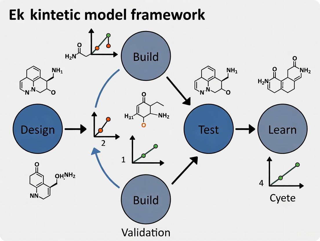
Design: Researchers define objectives for desired biological function and design parts or systems using domain knowledge and computational modeling [3]. In kinetic modeling, this corresponds to formulating mathematical representations of biological systems based on existing knowledge.

Build: DNA constructs are synthesized and assembled into plasmids or other vectors, then introduced into characterization systems [3]. For kinetic modeling, this phase involves implementing mathematical models in computational frameworks.

Test: Experimental measurement of engineered biological construct performance [3]. In modeling, this involves comparing predictions to empirical data.

Learn: Analysis of collected data compared to design objectives to inform subsequent design rounds [3]. This iterative refinement continues until desired function is achieved.

The Emerging LDBT Paradigm

Recent advances have prompted a paradigm shift from DBTL to LDBT (Learn-Design-Build-Test), where machine learning precedes design:

Learn: Machine learning models analyze existing biological data to detect patterns in high-dimensional spaces, enabling predictive design before physical construction [3]. Protein language models (ESM, ProGen) capture evolutionary relationships, while structural models (MutCompute, ProteinMPNN) predict sequences folding into specific backbones [3].

Design: Computational generation of biological designs informed by machine learning predictions rather than solely domain expertise [3]. This includes zero-shot prediction of functional sequences without additional training.

Build: Rapid construction using cell-free systems that express proteins without cloning steps, achieving high yields in hours rather than days [3].

Test: High-throughput functional characterization in cell-free systems, providing reproducible data under controlled conditions [3].

This reordering creates a feedback-efficient system that minimizes trial-and-error by frontloading computational learning, potentially achieving functional solutions in a single cycle rather than multiple iterations [3].

The Scientist's Toolkit: Essential Research Reagents and Solutions

Table 3: Key Research Reagents for Kinetic Modeling Validation

Reagent/Resource	Function/Application	Specific Examples
Cell-Free TX-TL Systems	Rapid protein expression without living cells	E. coli lysates, purified components [3]
Fluorescent Reporters	Quantitative measurement of biological activity	mCherry, GFP [4]
Bioluminescence Reporters	Highly sensitive, quantitative signaling	LuxCDEAB operon [4]
Machine Learning Models	Predictive protein design and optimization	ESM, ProGen, MutCompute, ProteinMPNN [3]
Specialized Plasmids	Genetic construct delivery and expression	pSEVA261 (medium-low copy number) [4]
Selection Markers	Maintenance of genetic constructs in hosts	Kanamycin resistance cassette [4]
Microfluidic Platforms	Ultra-high-throughput screening	DropAI droplet microfluidics [3]
Inducible Promoter Systems	Controlled gene expression testing	pTet/pLac with TetR/LacI regulators [4]

Case Study: Integration of Tracer Kinetics with Mechanistic Modeling

The Gadkar-Lu model of HDL metabolism exemplifies the integration of classical and modern approaches [1]. This model was formulated with explicit hypotheses tested quantitatively against multiple pharmacological perturbations:

• Upregulation of apoA1 synthesis
• Administration of reconstituted HDL
• Infusion of delipidated HDL
• CETP inhibition
• ABCA1 upregulation [1]

The model introduced a quantitative concept of HDL remodeling and apoA1 recycling that accounted for classic biphasic apoA1 kinetics previously reported by Ikewaki and colleagues [1]. When tested against Schwartz tracer time course data for lipoprotein cholesteryl ester kinetics, the model showed remarkable agreement in reported cholesterol fluxes despite differences in methodological approach [1]. This case study demonstrates how a single mechanistic model can account for both non-steady state perturbation data and steady-state tracer kinetic data, leveraging the unique capabilities of both modeling schools.

The legacy of the Berman-Levy collaboration and SAAM modeling extends far beyond their original applications in lipoprotein metabolism. Their work established foundational principles for combining experimental data with computational modeling that continue to evolve in modern systems pharmacology. The current convergence of linear, steady-state tracer kinetic modeling with nonlinear, mechanistic, non-steady state modeling represents a maturation of both traditions, each contributing unique strengths to the comprehensive understanding of biological systems [1].

This integration is particularly valuable in pharmaceutical development, where human and financial incentives encourage testing theories against as many different experimental protocols as possible [1]. The more validation tests a model passes, the greater confidence researchers have in its predictions. This comprehensive modeling approach ultimately benefits patients and provides competitive advantages to organizations that understand its value [1]. As kinetic modeling continues to evolve within the LDBT paradigm, the foundational principles established by Berman, Levy, and their contemporaries provide enduring guidance for relating mathematical representations to biological reality.

In the field of kinetic model framework validation within Design-Build-Test-Learn (DBTL) cycles, two dominant modeling philosophies provide complementary insights: classical Tracer Kinetics (TK) and Mechanistic Systems Biology (MSB) [1]. For decades, TK has been a powerful tool for quantifying metabolic fluxes in steady-state systems, using radioisotopes or stable isotopes to track molecular fate. In parallel, MSB has evolved to model the complex, nonlinear dynamics of biological systems by explicitly incorporating molecular mechanisms and regulatory structures [1] [5]. This guide provides an objective comparison of these approaches, detailing their performance characteristics, appropriate applications, and roles in modern pharmacological and metabolic engineering research.

Core Philosophical and Technical Differences

The fundamental distinction between these modeling approaches lies in their scope and objective. TK aims to describe systemic behavior by extracting composite rate constants from steady-state data, while MSB seeks to explain system behavior by mathematically representing underlying physical and biochemical mechanisms [1].

Tracer Kinetics operates on the principle of introducing traceable, non-perturbing amounts of labeled compounds into a system at steady state. The resulting data are analyzed, typically with linear differential equations and compartmental models, to determine kinetic parameters like production rates and clearance rate constants [1] [6]. Its power comes from the ability to distinguish between alternative physiological states—for example, determining whether elevated LDL-cholesterol stems from overproduction or impaired clearance [1]. However, this approach has a significant limitation: all molecular regulatory mechanisms remain hidden from view because, at steady state, transcriptional, translational, and allosteric controls are constant and thus invisible to the model [1].

Mechanistic Systems Biology explicitly represents these hidden controls. MSB models consist of large systems of nonlinear differential equations where every rate law includes known or hypothesized control mechanisms [1]. This allows upstream controllers to propagate changes to downstream processes, integrating multiple feedback mechanisms. These models are particularly valuable for analyzing physiological non-steady states, such as transitions from rest to exercise or metabolic responses to pharmacological perturbations [1]. In translational pharmaceutical research, TK models align with what the body does to a drug (pharmacokinetics), while MSB models align with what the drug does to the body (pharmacodynamics) [1].

The following diagram illustrates the fundamental differences in approach and information flow between these two modeling paradigms:

Comparative Performance Analysis

The table below summarizes the fundamental characteristics and performance metrics of TK and MSB approaches across key modeling dimensions.

Table 1: Fundamental Characteristics and Performance Comparison

Modeling Dimension	Tracer Kinetics (TK)	Mechanistic Systems Biology (MSB)
Primary Objective	Quantify metabolic fluxes & rate constants [1]	Elucidate molecular mechanisms & regulatory structures [1]
Mathematical Foundation	Linear algebra & linear differential equations [1]	Nonlinear differential equations [1]
System State Requirement	Steady state assumption [1]	Steady state or non-steady state [1]
Molecular Mechanisms	Hidden from view (lumped into rate constants) [1]	Explicitly represented in rate laws [1]
Regulatory Control	Invisible at steady state [1]	Explicitly modeled (allosteric, transcriptional, etc.) [1]
Predictive Scope	Limited to similar steady states [1]	Can predict responses to novel perturbations [1] [7]
Data Requirements	Tracer time-course data [1]	Multi-omics, kinetic parameters, perturbation data [1] [5]
Computational Intensity	Lower	Higher [1]

Experimental Applications and Validation Protocols

Representative Experimental Designs

The experimental protocols for TK and MSB differ significantly in design and objective, as shown in the comparative table below.

Table 2: Experimental Protocol Comparison

Protocol Component	Tracer Kinetics Experiment	Mechanistic Systems Biology Experiment
Experimental Goal	Identify which processes differ between states [1]	Validate hypothesized molecular mechanisms [1]
Subject Groups	Normal vs. abnormal phenotype (e.g., healthy vs. disease) [1]	Multiple groups with different mechanistic perturbations [1]
Intervention Type	Introduction of traceable label at steady state [1]	Targeted perturbations (genetic, pharmacological, environmental) [1] [7]
Key Measurements	Time-course of labeled metabolites [1]	Multi-omics data: metabolomics, fluxomics, proteomics [7] [5]
Validation Approach	Statistical comparison of rate constants between groups [1]	Ability to predict non-steady state responses to new perturbations [1]
Data Interpretation	Identifies where to look for mechanisms [1]	Proposes specific testable molecular mechanisms [1]

Performance in Practical Applications

In practical applications, each approach demonstrates distinct strengths and limitations, as evidenced by their implementation across various fields.

Table 3: Application Performance in Different Domains

Application Domain	Tracer Kinetics Performance	Mechanistic Systems Biology Performance
Lipoprotein Metabolism	50+ year history quantifying LDL production/clearance [1]	Emerging capability to model pharmacological perturbations [1]
Metabolic Engineering	Limited to steady-state flux analysis	Enables combinatorial pathway optimization in DBTL cycles [7]
Medical Imaging (DCE-MRI)	Standard models (e.g., Extended-Tofts) provide basic parameters [8] [9]	Advanced models (DP, TH) show superior diagnostic performance (AUC: 0.88 vs 0.73) [8]
Drug Development	Pharmacokinetics (what body does to drug) [1]	Systems pharmacology (what drug does to body) [1]
Nutritional Science	Whole-body nutrient utilization & requirements [5]	Multi-scale integration from molecular to physiological levels [5]

Integration in Modern DBTL Cycle Research

The most powerful contemporary approaches recognize the complementary strengths of TK and MSB, integrating them within iterative DBTL cycles. The following diagram illustrates how both modeling paradigms contribute to this integrated research framework:

In metabolic engineering, this integration is particularly advanced. Kinetic models of metabolic pathways serve as "digital twins" that simulate the effects of genetic modifications before physical strain construction [7] [10]. These models use ordinary differential equations parameterized with enzyme kinetic constants (Km, Vmax) to dynamically predict metabolite concentrations and pathway fluxes, capturing nonlinear effects and regulatory feedback missed by simpler steady-state models [7] [10]. The DBTL cycle becomes increasingly efficient as model predictions guide which strains to build and test, with experimental results refining model parameters in return [7].

Essential Research Toolkit

Successful implementation of TK and MSB approaches requires specific computational and experimental resources, as detailed in the table below.

Table 4: Essential Research Tools and Reagents

Tool/Reagent Category	Specific Examples	Research Function
Computational Modeling Software	SAAM, NONMEM, MONOLIX, specialized DCE analysis software [1] [8] [6]	Parameter estimation, compartmental modeling, nonlinear mixed-effects modeling [1] [6]
Tracer Compounds	Radioisotopes (¹⁴C, ³H, ¹²⁵I), stable isotopes (¹³C, ¹⁵N), PET tracers ([¹⁸F]FDG) [1] [11]	Metabolic pathway tracing, flux quantification, in vivo imaging [1]
Kinetic Parameters	Enzyme kinetic constants (Km, Vmax), inhibition constants, allosteric regulation parameters [7] [10]	Parameterizing mechanistic models, predicting pathway behavior [7]
Analytical Platforms	LC-MS/MS, GC-MS, NMR, MRI/PET scanners [7] [8] [5]	Quantifying metabolites, proteins, metabolic fluxes, and imaging parameters [7] [8]
Data Integration Tools	Multi-omics integration platforms, constraint-based modeling tools [7] [5] [12]	Integrating genomic, transcriptomic, proteomic, and metabolomic data [5] [12]

Tracer Kinetics and Mechanistic Systems Biology represent complementary rather than competing approaches to biological system modeling. TK excels at quantifying "what" is changing in steady-state systems, providing essential numerical constraints on metabolic fluxes. MSB aims to explain "why" systems behave as they do by explicitly representing underlying molecular mechanisms. The most powerful contemporary research frameworks integrate both approaches within iterative DBTL cycles, using TK to provide quantitative flux constraints and MSB to generate testable mechanistic hypotheses and predict system responses to novel perturbations. This synergistic approach accelerates discovery in metabolic engineering, drug development, and biomedical research by combining the descriptive power of TK with the predictive capability of MSB.

The Power and Limitations of Steady-State Assumptions in Biological Systems

The steady-state assumption represents a cornerstone simplification in the modeling and analysis of biological systems, from intracellular metabolic networks to enzymatic reactions. This principle, which posits that the concentrations of intermediate species remain constant over time, enables the tractable formulation of complex kinetic models that would otherwise be mathematically intractable. The validity and utility of this assumption are perpetually tested and refined within the iterative cycles of Design-Build-Test-Learn (DBTL), a framework central to modern biological engineering and kinetic model validation research.

While the steady-state approximation has driven significant advances, its application is bounded by intrinsic limitations. As noted in epistemological analyses of biological knowledge, "fundamental limitations arise from the structure imposed on the mathematical model by the nature of the science, in particular, its formal mathematical structure and its internal tractability" [13]. This article provides a comprehensive comparison of steady-state approaches across biological applications, examining their performance against more complex non-steady-state alternatives through experimental data, computational analyses, and their critical role in the DBTL cycle.

Theoretical Foundations of Steady-State Assumptions

Conceptual Framework and Mathematical Basis

The steady-state assumption fundamentally simplifies biological system analysis by asserting that the production and consumption rates of intermediate species are balanced. In mathematical terms, for a biological species with concentration ( C ), the steady-state condition is expressed as:

[ \dot C = 0 ]

This transforms differential equations that describe system dynamics into algebraic equations, dramatically reducing computational complexity. For instance, in the classic Michaelis-Menten enzyme kinetics model, applying steady-state to the enzyme-substrate complex concentration enables derivation of the familiar hyperbolic rate equation [14].

The theoretical justification for this assumption often rests on timescale separation – the concept that metabolic processes occur much faster than other cellular processes like gene expression [15]. This permits treating metabolism as being in a quasi-steady-state relative to slower cellular dynamics.

Expanding Beyond Traditional Applications

Recent mathematical frameworks have demonstrated that the steady-state assumption can be applied to a broader range of systems than previously recognized, including oscillating and growing systems where metabolites do not remain at constant levels at every time point, but where their production and consumption balance over longer periods [15]. This expanded perspective maintains the assumption's utility while acknowledging that "the average concentrations may not be compatible with the average fluxes" in such dynamic systems [15].

Table 1: Fundamental Types of Steady-State Assumptions in Biological Systems

Assumption Type	Mathematical Basis	Primary Application Domain	Key Requirement
Classical Quasi-Steady-State (sQSSA)	( \dot C = 0 ) for intermediate species	Michaelis-Menten enzyme kinetics	Low enzyme concentration relative to KM
Total Quasi-Steady-State (tQSSA)	( \dot{\bar{s}} = 0 ) for total substrate	Enzyme kinetics at higher enzyme concentrations	Low initial substrate concentration [14]
Metabolic Steady-State	( \frac{dM}{dt} = \text{Production} - \text{Consumption} = 0 )	Genome-scale metabolic modeling	Balance over relevant time period [15]
Operational Steady-State	Observable outputs constant over time	Biosensor performance characterization	Stable system parameters and inputs

Steady-State Approaches in the DBTL Cycle

The DBTL Framework in Biological Engineering

The Design-Build-Test-Learn (DBTL) cycle represents a systematic, iterative framework for biological engineering and model validation. In this context, steady-state assumptions play dual roles: they inform the design of biological constructs and provide the theoretical basis for testable models that can be validated experimentally.

Multiple iGEM teams have documented their use of iterative DBTL cycles to refine biological systems. For instance, the WIST team applied seven distinct DBTL cycles to optimize a cell-free arsenic biosensor, adjusting parameters such as plasmid concentration ratios and incubation times based on performance data [16]. Similarly, the LYON team employed DBTL cycles to engineer biosensors for detecting PFAS compounds, with steady-state performance characterization being a key testing component [4].

The Emergence of LDBT: A Learning-First Paradigm

Recent advances in machine learning are transforming the traditional DBTL approach. The proposed LDBT (Learn-Design-Build-Test) framework repositions learning at the beginning of the cycle, leveraging pre-trained models to inform initial designs [3] [17]. This paradigm shift enhances the role of steady-state principles, as they can be embedded within machine learning models that generate more effective starting designs, potentially reducing the number of iterations required to achieve functional biological systems.

The integration of cell-free transcription-translation (TX-TL) systems has further accelerated the Build-Test phases, enabling rapid empirical validation of steady-state assumptions and model predictions [3] [17]. This combination of computational and experimental advances creates a more efficient feedback loop for validating kinetic models incorporating steady-state approximations.

Comparative Analysis of Steady-State Methodologies

Enzyme Kinetics: sQSSA vs. tQSSA

The irreversible single-substrate, single-enzyme Michaelis-Menten reaction mechanism provides a classic test case for comparing steady-state approximations. The standard quasi-steady-state assumption (sQSSA) and total quasi-steady-state assumption (tQSSA) represent different mathematical approaches to simplifying this system.

The sQSSA assumes the enzyme-substrate complex is in quasi-steady-state with respect to the substrate, deriving the well-known Michaelis-Menten equation:

[ \dot s = -\frac{k2 e0 s}{K_M + s} ]

This reduction is based on the assumption of low initial reduced enzyme concentration (( e0/KM \ll 1 )) [14]. In contrast, the tQSSA, introduced by Borghans et al. (1996) and developed by Tzafriri (2003), replaces substrate ( s ) with total substrate ( \bar{s} = s + c ), proposing a modified equation that remains valid under broader conditions [14].

Recent mathematical analysis has clarified that the tQSSA's effectiveness is particularly "reasonable" under conditions of low initial substrate concentration (( s0/KM \ll 1 )) [14]. This work has helped resolve previous ambiguities about the tQSSA's range of validity, while also demonstrating its limitations at high substrate concentrations.

Table 2: Performance Comparison of Steady-State Approximations in Enzyme Kinetics

Parameter	Standard QSSA (sQSSA)	Total QSSA (tQSSA)	Linear tQSSA
Key Assumption	Low enzyme concentration (( e0/KM \ll 1 ))	Low initial substrate (( s0/KM \ll 1 )) [14]	Low initial substrate (( s0/KM \ll 1 )) [14]
Validity Range	Limited to classic Michaelis conditions	Broader parameter range	Specific to low ( s_0 )
Mathematical Complexity	Moderate	Higher	Simplified linear form
Prediction Accuracy	High within validity range	Generally improved over sQSSA	High for targeted conditions
Experimental Validation	Extensive	Growing support [14]	Recent computational support [14]

Metabolic Network Analysis

In metabolic engineering, the steady-state assumption enables flux balance analysis (FBA) by constraining metabolite concentrations to remain constant over time. This application demonstrates the power of steady-state approaches in handling genome-scale networks with hundreds or thousands of reactions.

The mathematical foundation for this application establishes that "the assumption of steady-state also applies to oscillating and growing systems without requiring quasi-steady-state at any time point" [15]. This represents a significant expansion of the concept's utility, acknowledging that steady-state can reflect a balance over longer time periods rather than instantaneous constancy.

However, this perspective also reveals limitations, as "the average concentrations may not be compatible with the average fluxes" in such systems [15]. This disconnect necessitates careful interpretation of steady-state results in dynamic biological contexts.

Biosensor Characterization and Optimization

The DBTL cycles documented by iGEM teams provide practical examples of steady-state principles in biosensor development. The WIST team's arsenic biosensor optimization involved characterizing steady-state performance metrics including sensitivity, specificity, and dynamic range across multiple iterations [16]. Their experimental protocols measured fluorescence output at equilibrium conditions to determine optimal plasmid concentration ratios (settling on a 1:10 sense-to-reporter ratio) and incubation parameters (standardizing at 37°C for 2-4 hours) [16].

The LYON team's PFAS biosensor development similarly employed steady-state fluorescence and bioluminescence measurements to characterize promoter activity and system performance [4]. Their approach highlights how steady-state measurements provide standardized metrics for comparing design iterations within the DBTL cycle.

Experimental Protocols and Methodologies

Protocol 1: Characterizing Enzyme Kinetics Under Steady-State Assumptions

Objective: Determine kinetic parameters (( KM ), ( V{max} )) using steady-state assumptions.

Methodology:

• Prepare enzyme solutions at varying concentrations, ensuring compatibility with sQSSA or tQSSA requirements
• Initiate reactions with substrate concentrations spanning expected ( K_M ) values
• Measure initial velocity rates under conditions where product accumulation is minimal (<5% substrate conversion)
• Record time-course data to verify steady-state conditions are maintained during measurements
• Fit data to appropriate steady-state model (Michaelis-Menten for sQSSA, modified equations for tQSSA)

Critical Considerations:

• Verify assumption validity through parameter consistency checks
• For tQSSA applications, ensure initial substrate concentration is sufficiently low [14]
• Account for enzyme concentration effects when applying sQSSA

Protocol 2: DBTL-Based Biosensor Performance Characterization

Objective: Optimize biosensor performance through iterative DBTL cycles with steady-state output measurements.

Methodology (adapted from iGEM WIST team [16]):

• Design: Specify desired sensitivity, dynamic range, and response time
• Build: Construct genetic circuits using standardized assembly methods
• Test:
  • Prepare master mix with cell-free lysate, polymerase, plasmids, and reporter molecules
  • Incubate at standardized temperature (e.g., 37°C) until steady-state response is achieved
  • Measure fluorescence/luminescence output across analyte concentrations
  • Determine signal-to-noise ratio and leakiness
• Learn: Analyze performance data to inform next design iteration

Technical Refinements:

• Implement simultaneous addition of all reaction components to minimize variability
• Use kinetic reading over extended periods (e.g., 90 minutes) to identify response plateaus
• Systematically vary component ratios (e.g., plasmid concentrations) to optimize dynamic range

Limitations and Boundary Conditions

Mathematical and Conceptual Constraints

The power of steady-state assumptions is counterbalanced by intrinsic limitations. As noted in analyses of biological knowledge, "fundamental limitations arise from the structure imposed on the mathematical model by the nature of the science" [13]. These include:

Mathematical Complexity: As biological models increase in size and complexity, deriving closed-form analytic solutions becomes increasingly difficult. Examples include "deriving limit cycles and mean first passage times in Markovian models of gene regulatory networks" [13]. This complexity often necessitates model reduction, which increases stochasticity and decreases predictability.

Experimental Constraints: Measurement technologies limit our ability to fully parameterize complex models, leading to systems with "latent variables" that introduce apparent stochasticity [13]. The p53 network example demonstrates how unobserved variables (like DNA damage status) can create seemingly stochastic behavior in deterministic systems [13].

Knowledge Discovery Limitations: The steady-state assumption may obscure transient dynamics that provide crucial insights into system behavior, particularly in oscillating systems or those with multi-timescale processes.

Practical Limitations in Application

Timescale Mismatch: The steady-state assumption breaks down when the timescales of interacting processes do not separate cleanly. This is particularly problematic in systems combining fast metabolic processes with slower genetic regulation.

Context Dependence: As demonstrated in DBTL cycles, optimal parameters for steady-state performance are often highly specific to experimental context. The WIST team found that plasmid concentration ratios, incubation times, and temperature all required context-specific optimization [16].

Computational Trade-offs: While steady-state approaches reduce computational complexity, they may sacrifice accuracy in dynamic systems. Recent machine learning approaches like DLRN (Deep Learning Reaction Network) have emerged to address some limitations, demonstrating "comparable performance and, in part, even better than a classical fitting analysis" for analyzing complex kinetic data [18].

Computational Advances and Emerging Alternatives

Machine Learning-Enhanced Kinetic Modeling

Recent computational advances are transforming kinetic modeling beyond traditional steady-state approaches. The DLRN framework uses deep neural networks with Inception-Resnet architecture to analyze time-resolved data and identify kinetic models, including their parameters and pathways [18]. This approach demonstrates particular utility for complex multi-step processes like ATP-driven DNA dynamics and enzymatic reaction networks [18].

Similarly, the UniKP framework leverages pretrained language models to predict enzyme kinetic parameters (( k{cat} ), ( KM ), and ( k{cat}/KM )) from protein sequences and substrate structures [19]. This unified framework shows remarkable improvement over previous prediction methods, with a 20% improvement in prediction accuracy for ( k_{cat} ) values compared to earlier approaches [19].

Hybrid Approaches for Complex Systems

For systems where pure steady-state assumptions are insufficient but complete dynamic modeling is intractable, hybrid approaches offer promising alternatives. These include:

Multi-Timescale Modeling: Segmenting systems based on characteristic timescales and applying appropriate approximations to each segment.

Piecewise Steady-State Analysis: Applying steady-state assumptions to specific subsystems or during certain operational phases.

Physics-Informed Machine Learning: Integrating physical principles with data-driven approaches to maintain biological plausibility while leveraging pattern recognition capabilities [3].

Table 3: Computational Tools for Kinetic Modeling Beyond Steady-State

Tool/Framework	Methodology	Application Scope	Performance Advantages
DLRN [18]	Deep learning (Inception-Resnet)	Chemical reaction networks from time-resolved data	Identifies complex kinetic models with high accuracy (83.1% Top 1 accuracy)
UniKP [19]	Pretrained language models (ProtT5, SMILES)	Enzyme kinetic parameter prediction	20% improvement in ( k_{cat} ) prediction accuracy over previous tools
EF-UniKP [19]	Two-layer ensemble model	Enzyme kinetics with environmental factors	Robust prediction considering pH and temperature effects
LDBT Framework [3] [17]	Machine learning-first DBTL	Biological design automation	Accelerates design process through zero-shot predictions

The Scientist's Toolkit: Essential Research Reagents and Solutions

Table 4: Key Research Reagents and Experimental Materials

Reagent/Material	Function	Application Examples
Cell-Free TX-TL Systems	In vitro transcription-translation for rapid testing	Protein expression without cloning steps; biosensor characterization [3] [17]
Plasmid Vectors (e.g., pSEVA261)	Genetic construct delivery	Controlled gene expression; biosensor assembly [4]
Reporter Systems (Luciferase, GFP, mCherry)	Quantitative output measurement	Promoter activity assessment; system performance quantification [4]
Microplate Readers with Kinetic Capabilities	Time-resolved fluorescence/luminescence measurement	Steady-state verification; dynamic response characterization [16]
Specialized Buffers with Cofactor Supplements	Optimized reaction environments	Maintaining enzyme activity; supporting cell-free reactions [16]

The steady-state assumption remains a powerful tool in biological system analysis, providing essential simplification that enables the study of otherwise intractable systems. Its continued utility within DBTL frameworks demonstrates its enduring value for biological engineering and kinetic model validation. However, researchers must remain cognizant of its limitations and the boundary conditions for its application.

Emerging computational approaches, particularly machine learning frameworks like DLRN and UniKP, are extending our capabilities beyond traditional steady-state methods. These tools, combined with high-throughput experimental platforms like cell-free TX-TL systems, are creating new paradigms for biological design and analysis. The evolution from DBTL to LDBT cycles represents a fundamental shift toward learning-driven biological engineering, where steady-state principles inform rather than constrain biological design.

As biological complexity continues to challenge our modeling capabilities, the judicious application of steady-state assumptions – with clear understanding of their power and limitations – will remain essential for advancing our understanding and engineering of biological systems.

Visual Appendix: Signaling Pathways and Workflows

Simplified p53 Regulatory Network

DBTL Cycle Workflow

Michaelis-Menten Reaction Mechanism

Integrating Linear Pharmacokinetics with Nonlinear Pharmacodynamic Models

The integration of Linear Pharmacokinetics (PK) with Nonlinear Pharmacodynamic (PD) models represents a critical frontier in modern drug development. This integration allows researchers to quantitatively link a drug's concentration-time profile (PK) to its pharmacological effect (PD), even when the relationship between exposure and response is complex and saturable [20]. Within the framework of kinetic model validation research, the Design-Build-Test-Learn (DBTL) cycle has emerged as a powerful, iterative paradigm for optimizing this integration [7] [21]. This guide provides a comparative analysis of linear PK and nonlinear PD models, detailing their respective roles, the experimental data required for their development, and their application within a DBTL cycle to enhance the efficiency and predictive power of therapeutic development.

The core challenge this integration addresses is the frequent disconnect between a drug's predictable, dose-proportional exposure in the body (linear PK) and its often disproportionate, saturable biological effect (nonlinear PD). By combining these elements into a unified mathematical model, scientists can make more informed decisions on dosing, patient selection, and trial design, ultimately streamlining the path from discovery to clinic [22] [20].

Comparative Foundations: Linear PK vs. Nonlinear PD

Core Principles of Linear Pharmacokinetics

Linear pharmacokinetics are characterized by processes where the parameters governing drug absorption, distribution, and elimination are independent of the drug's concentration and time [23]. The most crucial feature is constant clearance, where the rate of drug elimination is directly proportional to its concentration in plasma [23] [24].

• Dose Proportionality: A fundamental principle of linear PK is that the Area Under the Curve (AUC), representing total drug exposure, is directly proportional to the administered dose. Doubling the dose results in a doubling of the AUC [23].
• Schedule Independence: The total drug exposure (AUC) is not affected by changes in the administration schedule. For example, the AUC from a single large bolus dose is equivalent to the combined AUC from multiple smaller doses or a continuous infusion of the same total dose [23].
• Constant Half-Life: The elimination half-life remains constant, regardless of the drug's concentration. This leads to a predictable, exponential decay in plasma concentration over time [23].

Core Principles of Nonlinear Pharmacodynamics

In contrast, nonlinear pharmacodynamics describe a scenario where the magnitude of the drug's effect does not change in direct proportion to its concentration at the effect site. This nonlinearity is often due to the saturation of biological systems [25].

• Saturable Receptors or Pathways: The drug's effect may plateau at higher concentrations once all target receptors are occupied or a downstream signaling pathway is fully activated.
• Signal Transduction Amplification: Biological systems can amplify a signal, meaning a small increase in target engagement can lead to a disproportionately large biological effect.
• Indirect Mechanisms of Action: The drug may act through complex, multi-step mechanisms (e.g., inhibition of protein synthesis or cell cycle arrest) where the observed effect is delayed and not directly proportional to the instantaneous plasma concentration.

The table below summarizes the key distinctions between these two concepts.

Table 1: Fundamental Characteristics of Linear PK and Nonlinear PD Models

Feature	Linear Pharmacokinetics	Nonlinear Pharmacodynamics
Core Relationship	Parameters are independent of dose and time [23]	Effect is not directly proportional to drug concentration at the site of action
Dose-Exposure/Effect	AUC is proportional to dose [23]	Effect plateaus at high concentrations (Emax model)
Key Model Parameter	Clearance (CL) - constant [23] [24]	EC50 (potency) & Emax (efficacy)
Governing Equation	Rate of Elimination = CL × Cp [24]	E = (Emax × C) / (EC50 + C) (Basic Emax model)
Primary Cause	Unsaturated elimination pathways (enzymes, transporters)	Saturation of target binding, signal transduction, or physiological systems
Clinical Implication	Predictable exposure; simple dose scaling	Complex dose optimization; risk of diminished returns or increased toxicity at high doses

The DBTL Cycle Framework for Model Integration

The DBTL cycle provides a structured, iterative framework for developing and validating integrated PK/PD models. Its power lies in using data from one cycle to inform and improve the design of the next, creating a continuous feedback loop for model refinement [7]. The workflow of this cycle and the specific role of PK/PD integration within it are visualized below.

Diagram 1: The DBTL cycle workflow, highlighting the integration of PK and PD data into a unified model during the 'Learn' phase.

Phase 1: Design

The "Design" phase involves defining the integrated PK/PD model's mathematical structure and planning the experiments that will generate data for its parameterization [21]. For a model integrating linear PK with nonlinear PD, the structural model might be:

• PK Sub-model: A one- or two-compartment linear model with first-order elimination [23].
• PD Sub-model: A direct or indirect Emax model linking the plasma or effect-site concentration from the PK model to the observed effect [20].

A critical activity in this phase is Design of Experiments (DoE), which aims to maximize information gain while minimizing experimental effort. For a pathway with multiple factors, Resolution IV fractional factorial designs have been shown to effectively identify optimal conditions and guide subsequent optimization cycles without the prohibitive cost of a full factorial approach [26].

Phase 2: Build

In the "Build" phase, the planned experiments are executed. This involves:

• Synthesizing the drug compound or biologic.
• Preparing the in vitro (e.g., cell cultures, tissue preparations) or in vivo (e.g., animal models) systems.
• Implementing the dosing regimens and sampling schedules defined in the DoE [7].

Phase 3: Test

The "Test" phase is dedicated to data collection. High-quality, well-timed data is crucial for robust model parameterization [23] [21]. Key activities include:

• PK Sampling: Collecting serial blood/plasma samples at precise times to characterize the drug's concentration-time profile.
• PD Monitoring: Measuring the pharmacological response(s) concurrently with PK sampling. This can range from biomarker quantification (e.g., protein levels, metabolic products) to clinical endpoint assessment [20].

Phase 4: Learn

The "Learn" phase is where PK and PD data are integrated. The collected data are used to:

• Parameterize the Model: Estimate the key parameters of both the PK (e.g., Clearance, Volume of distribution) and PD (e.g., EC50, Emax) sub-models using nonlinear regression or population modeling techniques [20].
• Validate the Model: Assess the model's predictive performance against a validation dataset or through statistical diagnostics [21].
• Generate Hypotheses: The validated model is used to simulate new scenarios, such as different dosing regimens, which then inform the "Design" of the next DBTL cycle [7].

Experimental Protocols and Data for Model Development

Protocol for Characterizing Linear PK

Objective: To determine the fundamental PK parameters (AUC, CL, V, t½) and confirm linear kinetics over the intended therapeutic dose range.

Methodology:

• Study Design: A single-dose, multi-level escalating dose study in a relevant pre-clinical model (e.g., rodent, non-human primate) or human participants. Doses should span the anticipated therapeutic range.
• Dosing & Sampling: Administer the drug via the intended clinical route (e.g., IV bolus, oral). Collect serial blood samples at pre-defined times post-dose (e.g., 0.25, 0.5, 1, 2, 4, 8, 12, 24 hours).
• Bioanalysis: Use a validated analytical method (e.g., LC-MS/MS) to quantify drug concentrations in each plasma sample [27].
• Data Analysis:
  • Calculate AUC for each dose level using non-compartmental analysis (NCA).
  • Plot AUC vs. Dose. A linear relationship with a high coefficient of determination (R² > 0.95) confirms dose proportionality [23].
  • Calculate clearance (CL = Dose / AUC) and other parameters. Consistent CL values across dose levels confirm linearity [23].

Protocol for Characterizing Nonlinear PD

Objective: To establish the quantitative relationship between drug concentration and pharmacological effect and parameterize a nonlinear Emax model.

Methodology:

• Study Design: An in vivo efficacy study or an in vitro cell-based assay where the biological effect can be measured across a wide concentration range.
• Intervention & Sampling: Expose the system to a range of drug concentrations. For in vivo studies, this may involve different dose groups. Measure the PD endpoint (e.g., enzyme activity, cell proliferation, pain response) at each concentration. Concurrent PK sampling is ideal to link effect to actual exposure.
• Data Analysis:
  • Plot the measured effect against the corresponding drug concentration.
  • Fit the data to a sigmoidal Emax model: E = E0 + (Emax × C^h) / (EC50^h + C^h), where E0 is the baseline effect, Emax is the maximum effect, EC50 is the concentration producing 50% of Emax, and h is the Hill coefficient accounting for sigmoidicity.
  • Use nonlinear regression software to estimate the parameters Emax, EC50, and h.

Table 2: Key Parameters from PK and PD Experimental Protocols

Parameter	Description	Interpretation	Typical Units
AUC	Area Under the plasma Concentration-time curve	Total drug exposure	h*μg/mL
CL	Clearance	Volume of plasma cleared of drug per unit time; constant in linear PK	L/h
EC50	Drug concentration producing 50% of maximal effect	Measure of drug potency; lower EC50 = higher potency	μg/mL or nM
Emax	Maximum achievable effect	Measure of drug efficacy	Varies (e.g., % inhibition, score)
Hill Coefficient (h)	Steepness of the concentration-effect curve	h > 1 suggests cooperative binding	Unitless

Integrated PK/PD Modeling and the Scientist's Toolkit

The final step is to mathematically link the PK and PD components. For a model with linear PK and direct-effect nonlinear PD, the workflow is illustrated below.

Diagram 2: Logical flow of an integrated PK/PD model, where the output of the linear PK model serves as the input to the nonlinear PD model.

Successful implementation of this research requires a combination of computational tools, experimental reagents, and analytical services.

Table 3: Essential Research Reagent Solutions and Tools

Item Name	Category	Primary Function in PK/PD Research
LC-MS/MS System	Analytical Instrument	High-sensitivity quantification of drug concentrations in biological matrices (plasma, tissue) for PK analysis [27].
Validated Bioanalytical Assay	Method	Ensures accuracy, precision, and reproducibility of concentration measurements, which is critical for model parameterization [27].
PBPK/PD Software (e.g., Simcyp)	Computational Tool	Mechanistic, physiologically-based modeling platform to simulate and scale PK/PD from pre-clinical to human populations [20].
Population PK/PD Software (e.g., NONMEM)	Computational Tool	Used for parameterizing models using sparse, variable data from clinical populations, quantifying inter-individual variability [22] [24].
Michaelis-Menten Enzyme Kinetics Assay	Reagent/Biochemical Kit	Characterizes saturable metabolic pathways in vitro, providing initial estimates for Vmax and Km that may explain nonlinear PK [25].
High-Throughput Screening Systems	Platform	Enables rapid testing of PD effects (e.g., on-cell target engagement) across a wide concentration range for Emax model building [7].

The strategic integration of linear pharmacokinetic models with nonlinear pharmacodynamic frameworks provides a powerful, quantitative approach to understanding and predicting drug behavior. When embedded within a rigorous DBTL cycle, this integrated approach transforms drug development from an empirical, trial-and-error process into a rational, iterative learning system. By objectively comparing the principles, data requirements, and modeling outputs of linear PK and nonlinear PD, researchers can more effectively design experiments, build predictive models, and ultimately accelerate the development of safer and more effective therapeutics.

The Rise of Systems Pharmacology in Contemporary Drug Development

The landscape of drug development is undergoing a fundamental transformation, moving away from traditional reductionist approaches toward a more holistic, systems-level framework. Systems pharmacology represents this paradigm shift, integrating computational modeling, multiscale biological data, and quantitative methods to understand complex interactions between drugs, biological networks, and disease processes. This approach addresses the critical limitations of single-target drug discovery, which has faced high attrition rates in clinical trials due to inadequate efficacy and unexpected toxicity in complex diseases [28]. The emergence of systems pharmacology coincides with growing recognition that most diseases, particularly cancer, neurodegenerative disorders, and metabolic syndromes, involve dysregulated networks rather than isolated molecular defects, necessitating therapeutic strategies that target multiple pathways simultaneously [29] [28].

The foundation of modern systems pharmacology rests upon several key technological advancements: the availability of large-scale biological datasets ("omics" technologies), sophisticated computational modeling platforms, and artificial intelligence (AI) applications. According to recent analyses, the integration of these elements through Model-Informed Drug Development (MIDD) frameworks can significantly shorten development timelines and reduce costs—estimated savings of $5 million and 10 months per development program based on Pfizer data [30]. The field has matured to the point where regulatory agencies like the FDA and EMA are increasingly accepting these approaches, with a notable rise in submissions leveraging Quantitative Systems Pharmacology (QSP) models over the past decade [31] [30].

Methodological Frameworks: DBTL Cycles and Kinetic Modeling

The Design-Build-Test-Learn (DBTL) Cycle

At the core of modern systems pharmacology lies the iterative Design-Build-Test-Learn (DBTL) cycle, a systematic framework for optimizing therapeutic interventions. This engineering-inspired approach enables researchers to continuously refine hypotheses and designs based on experimental feedback [7] [32]. The DBTL cycle consists of four interconnected phases:

• Design: Researchers identify targets and plan interventions using computational tools and prior knowledge
• Build: Genetic constructs or drug candidates are created using synthetic biology and automated platforms
• Test: High-throughput experiments evaluate the performance of designs in biological systems
• Learn: Data analysis and machine learning extract insights to inform the next design cycle

Recent advancements have introduced "knowledge-driven" DBTL cycles that incorporate upstream in vitro investigations to accelerate the learning phase. For instance, researchers developing dopamine-producing Escherichia coli strains used cell-free protein synthesis systems to test enzyme expression levels before implementing changes in living organisms, significantly reducing development iterations [32]. This approach enabled a 2.6 to 6.6-fold improvement in dopamine production over existing methods by systematically optimizing pathway enzyme levels through ribosome binding site engineering [32].

Kinetic Modeling Frameworks

Kinetic models provide the mathematical foundation for systems pharmacology by describing biological systems through ordinary differential equations that capture the dynamics of metabolic and signaling pathways [7]. These mechanistic models differ from purely statistical approaches by incorporating biological constraints and prior knowledge, enabling more accurate predictions of system behavior under perturbation.

A key advantage of kinetic models is their ability to simulate counterintuitive pathway behaviors that challenge conventional wisdom. For example, in metabolic engineering, simply increasing enzyme concentrations does not always enhance flux toward desired products; in some cases, it can deplete substrates and reduce output—a phenomenon that can be predicted and avoided through kinetic modeling [7]. These models create virtual testbeds for exploring "what-if" scenarios before committing to costly experimental work.

Table 1: Comparison of Modeling Approaches in Drug Development

Modeling Approach	Key Features	Primary Applications	Limitations
Quantitative Systems Pharmacology (QSP)	Multiscale, mechanistic, incorporates pathophysiology	Target identification, dose optimization, clinical trial simulation	High computational demand, requires extensive biological knowledge
Physiologically Based Pharmacokinetics (PBPK)	Organ-level resolution, species scaling	ADME prediction, drug-drug interactions, first-in-human dosing	Limited pharmacodynamic components
Population PK/PD	Statistical, accounts for variability	Exposure-response analysis, dosing individualization	Often empirical rather than mechanistic
Quantitative Structure-Activity Relationship (QSAR)	Ligand-based, uses molecular descriptors	Compound screening, toxicity prediction	Limited to similar chemical scaffolds

Comparative Analysis: Traditional vs. Network Pharmacology

The transition from traditional to network pharmacology represents more than just technological advancement—it constitutes a fundamental shift in how we conceptualize drug action and therapeutic intervention. Classical pharmacology has operated predominantly on a "one-drug-one-target" model that emerged from receptor theory, focusing on highly specific molecular interactions between drugs and their protein targets [28]. While this approach has produced successful treatments for infectious diseases and conditions with well-defined molecular etiology, it has proven inadequate for addressing complex multifactorial diseases characterized by redundant pathways and network-level dysregulation [28].

Network pharmacology, in contrast, embraces the complexity of biological systems by examining drug actions within interconnected molecular networks. This paradigm leverages omics technologies, bioinformatics, and computational modeling to identify multi-target strategies that can produce more robust therapeutic effects with reduced side effects [28]. The distinction between these approaches extends throughout the drug development process, from target identification to clinical application.

Table 2: Traditional Pharmacology vs. Network Pharmacology

Feature	Traditional Pharmacology	Network Pharmacology
Targeting Approach	Single-target	Multi-target / network-level
Disease Suitability	Monogenic or infectious diseases	Complex, multifactorial disorders
Model of Action	Linear (receptor-ligand)	Systems/network-based
Risk of Side Effects	Higher (off-target effects)	Lower (network-aware prediction)
Failure in Clinical Trials	Higher (60-70%)	Lower due to pre-network analysis
Technological Tools Used	Molecular biology, pharmacokinetics	Omics data, bioinformatics, graph theory
Personalized Therapy	Limited	High potential (precision medicine)

The therapeutic advantages of network approaches are particularly evident in oncology, where resistance to single-target therapies remains a major clinical challenge. For example, QSP models in immuno-oncology have successfully identified combination therapies that simultaneously target tumor cells and modulate immune responses, leading to improved anti-tumor efficacy in scenarios where monotherapies fail [29]. These models capture the dynamic interactions between tumor biology, drug pharmacokinetics, and immune system components, enabling more predictive simulation of treatment outcomes across patient populations.

Key Technologies and Research Solutions

Computational and Modeling Platforms

The implementation of systems pharmacology relies on sophisticated software platforms that enable the construction, simulation, and analysis of complex biological networks. The MATLAB/SimBiology environment has emerged as a popular choice for QSP modeling, providing tools for building dynamical systems models, estimating parameters from experimental data, and running virtual patient simulations [29] [33]. Other platforms like R-based packages (nlmixr, mrgsolve, RxODE) and specialized tools such as Cell Collective offer complementary capabilities for different aspects of model development and analysis [29].

These computational environments support the QSP workflow which typically involves: (1) model building using diagrammatic or programmatic interfaces, (2) importing and visualizing experimental data, (3) parameter estimation through optimization algorithms, (4) simulation of "what-if" scenarios, (5) sensitivity analysis to identify key pathways, and (6) virtual patient generation to explore population heterogeneity [33]. This workflow enables researchers to move iteratively between experimental data and model refinement, progressively improving the predictive power of their simulations.

Experimental and Reagent Solutions

The computational aspects of systems pharmacology are grounded in experimental biology, with specific reagent systems and research tools playing critical roles in model development and validation.

Table 3: Essential Research Reagents and Platforms in Systems Pharmacology

Reagent/Platform	Function	Application Example
Cell-free protein synthesis (CFPS) systems	Test enzyme expression and pathway function	In vitro optimization of dopamine pathway [32]
Ribosome Binding Site (RBS) libraries	Fine-tune gene expression levels	Metabolic pathway optimization in E. coli [32]
Promoter libraries	Vary transcription rates	Combinatorial pathway optimization [7]
UTR Designer tools	Modulate translation efficiency	RBS engineering for synthetic biology [32]
Kinetic model platforms (SKiMpy)	Simulate metabolic pathways	Predicting flux in engineered strains [7]
High-throughput screening automation	Rapid testing of genetic variants	DBTL cycle implementation [7] [32]

Artificial Intelligence and Machine Learning Integration

The integration of artificial intelligence (AI) and machine learning (ML) with systems pharmacology creates a powerful synergy between mechanistic understanding and data-driven pattern recognition [34]. ML algorithms excel at identifying complex patterns in high-dimensional data, while QSP models provide biological context and mechanistic constraints. This combination is particularly valuable in areas such as target prediction, where ML can screen vast chemical spaces while QSP models assess the system-level consequences of target modulation [34].

Leading AI-driven drug discovery companies have demonstrated the practical potential of these integrated approaches. Exscientia, for example, has developed an automated platform that combines AI-based compound design with robotic synthesis and testing, achieving approximately 70% faster design cycles while requiring 10-fold fewer synthesized compounds than traditional medicinal chemistry [35]. Similarly, Insilico Medicine reported advancing an idiopathic pulmonary fibrosis drug from target discovery to Phase I trials in just 18 months—significantly faster than the typical 5-year timeline for conventional approaches [35].

Case Studies and Experimental Validation

Dopamine Production in E. coli via Knowledge-Driven DBTL

A recent study demonstrates the power of combining kinetic modeling with experimental validation in optimizing microbial production of dopamine [32]. Researchers implemented a knowledge-driven DBTL cycle that began with in vitro testing in cell lysate systems to determine optimal enzyme ratios before moving to live cells. This approach resulted in a high-yielding dopamine strain producing 69.03 ± 1.2 mg/L, representing a 2.6 to 6.6-fold improvement over previous reports [32].

The experimental protocol involved:

• Strain engineering: Creating E. coli FUS4.T2 with enhanced L-tyrosine production
• Pathway construction: Introducing heterologous genes hpaBC and ddc under inducible control
• In vitro testing: Using cell lysate systems to determine optimal enzyme expression levels
• RBS library construction: Generating 16 variants with modified Shine-Dalgarno sequences
• High-throughput screening: Evaluating dopamine production across variants
• Model refinement: Incorporating results into kinetic models for further prediction

This case highlights how upstream in vitro investigation can guide subsequent in vivo engineering, reducing the number of DBTL cycles required to achieve performance targets.

Immuno-Oncology Applications

Quantitative Systems Pharmacology has shown particular promise in immuno-oncology, where it helps unravel the complex interactions between tumors, immune cells, and therapeutic agents. Recent QSP models have incorporated tumor heterogeneity, immune cell trafficking, and checkpoint inhibitor mechanisms to simulate patient responses to immunotherapies [29]. These models have identified combination therapies that simultaneously target multiple pathways in the cancer-immunity cycle, leading to improved anti-tumor efficacy compared to monotherapies.

One published QSP model focused on triple-negative breast cancer successfully predicted the efficacy of atezolizumab and nab-paclitaxel combination therapy by capturing the dynamics of immune cell infiltration and tumor cell killing [29]. The model provided insights into optimal dosing schedules that would be difficult to determine through clinical trials alone, demonstrating how QSP can guide clinical translation of combination immunotherapies.

Signaling Pathways and Workflow Visualization

The implementation of systems pharmacology relies on clearly defined workflows and pathway representations. The following diagrams illustrate key processes in systems pharmacology approaches.

DBTL Cycle Workflow

Dopamine Biosynthesis Pathway

Future Perspectives and Challenges

As systems pharmacology continues to evolve, several emerging trends and challenges will shape its trajectory. The integration of multi-omics data (genomics, transcriptomics, proteomics, metabolomics) with QSP models promises to enhance their predictive power and biological relevance [28]. Similarly, the creation of virtual patient populations through QSP modeling addresses a critical need in drug development, particularly for rare diseases and pediatric populations where clinical trials are ethically or practically challenging [30].

Significant challenges remain, including the need for standardized model qualification methods, improved data quality and accessibility, and broader organizational acceptance of model-informed approaches [31] [29]. The field must also address technical hurdles related to model scalability and computational efficiency as systems representations become increasingly comprehensive.

Perhaps most importantly, the ultimate validation of systems pharmacology will come through clinical translation—demonstrating that model-informed therapeutic strategies actually improve patient outcomes. While AI-designed molecules are advancing through clinical trials, none have yet received regulatory approval, raising questions about whether these approaches deliver better success or merely faster failures [35]. Ongoing clinical studies will determine the real-world impact of systems pharmacology on drug development efficiency and therapeutic success rates.

Despite these challenges, the continued expansion of systems pharmacology appears inevitable given the compelling economic and scientific value proposition. As one industry analysis concluded: "QSP is no longer an emerging methodology; it is becoming the new standard in drug development" [30]. This transition represents not just a technological shift but a fundamental reimagining of how we understand and intervene in biological systems for therapeutic benefit.

Implementing Kinetic DBTL Frameworks: Practical Applications Across Biomedical Domains

Mechanistic Kinetic Models as In Silico Testbeds for DBTL Cycle Optimization

In the field of synthetic biology and metabolic engineering, the Design-Build-Test-Learn (DBTL) cycle serves as the fundamental engineering paradigm for developing efficient microbial cell factories. Mechanistic kinetic models have emerged as powerful in silico testbeds that provide a computational framework to simulate and optimize these iterative cycles before embarking on costly experimental work. These mathematical models simulate the dynamic behavior of biological systems, enabling researchers to predict pathway performance, identify metabolic bottlenecks, and evaluate optimization strategies under controlled virtual conditions. The integration of these models creates a simulated biological environment where different experimental designs, machine learning approaches, and optimization algorithms can be rigorously tested and validated, thereby accelerating the development of robust microbial strains for chemical production [36] [37] [38].

The broader thesis context of kinetic model framework validation research positions these computational tools as essential components for establishing predictive biological engineering. By providing a ground-truth simulation environment, kinetic models enable direct comparison between predicted and actual biological behavior, facilitating the validation of DBTL frameworks under conditions that mimic real-world biological complexity while offering complete parameter control and reduced experimental variance [36]. This review objectively compares the performance of various DBTL optimization strategies evaluated through kinetic modeling approaches, providing researchers with evidence-based guidance for selecting appropriate methods for their specific applications.

Kinetic Modeling Frameworks for DBTL Validation

Fundamental Framework Architecture

Mechanistic kinetic modeling frameworks for DBTL cycle validation typically employ ordinary differential equation (ODE) systems that mathematically represent the biochemical reactions within metabolic pathways. These frameworks simulate the dynamic flux of metabolites through engineered pathways, capturing complex regulatory interactions and enzyme kinetics that influence overall production yields. The foundational structure comprises mass-action kinetics and enzyme catalytic mechanisms that collectively determine pathway dynamics and emergent properties [36] [37].

The kinetic model framework introduced by van Ladereen et al. exemplifies this approach, implementing a virtual seven-gene pathway with parameters derived from experimentally validated enzyme kinetics [36] [37] [38]. This framework specifically simulates the performance of full factorial strain libraries and serves as a benchmark for comparing reduced experimental designs. The model incorporates biological noise and experimental variance parameters, enabling researchers to evaluate optimization methods under conditions that mirror real-world laboratory challenges, including measurement error and biological variability that can significantly impact algorithm performance and experimental conclusions [26] [36].

Key Framework Components and Capabilities

Table 1: Core Components of Kinetic Modeling Frameworks for DBTL Validation

Component	Function	Implementation Example
Virtual Pathway	Serves as ground truth for method validation	Seven-gene pathway with known optimal expression combination [26] [36]
Noise Integration	Mimics experimental variance in biological data	Incorporation of Gaussian noise models for measurement error [26] [36]
Performance Metrics	Quantifies optimization algorithm effectiveness	Production yield, convergence speed, resource utilization [26] [36] [37]
Experimental Design Simulator	Tests different factor combinations and sample sizes	Comparison of full factorial, fractional factorial, and Plackett-Burman designs [26]
Machine Learning Interface	Enables algorithm training and prediction testing	Integration with random forest, gradient boosting, and linear models [36] [37]

The simulated DBTL cycle framework employs a modular architecture that separately implements each phase of the engineering cycle. The design phase incorporates algorithms for selecting genetic parts and expression levels, while the build phase simulates strain construction with predictable success rates. The test phase generates synthetic analytical data with configurable noise profiles, and the learn phase applies machine learning algorithms to extract patterns and recommend improved designs for subsequent cycles [36] [37] [38]. This comprehensive approach enables researchers to systematically evaluate how different strategies at each DBTL phase contribute to overall optimization efficiency, providing insights that would be prohibitively expensive or time-consuming to obtain through purely experimental approaches.

Comparative Analysis of DoE Methods via Kinetic Models

Experimental Protocol for DoE Comparison

Kinetic models enable rigorous comparison of Design of Experiment (DoE) methods through a standardized protocol that simulates pathway optimization campaigns. The fundamental approach involves implementing a virtual seven-gene pathway based on mechanistic enzyme kinetics, which serves as a biological ground truth [26]. Researchers then simulate the construction and testing of strain libraries representing different experimental designs, including full factorial, resolution V, IV, III, and Plackett-Burman (PB) designs [26]. Each simulated design is evaluated based on its ability to identify the optimal strain configuration while minimizing the number of experiments required.

The testing protocol incorporates biological realism by introducing experimental noise and missing data points into the synthetic datasets, reflecting challenges inherent to actual biological experiments [26]. Performance metrics are quantified, including the success rate in identifying top-producing strains, robustness to noise, and efficiency in experimental resource utilization. The resulting data enables direct comparison of DoE methods under identical biological conditions, providing objective guidance for selecting appropriate experimental designs for pathway optimization projects with different constraints and objectives.

Quantitative Performance Comparison of DoE Methods

Table 2: Performance Comparison of Experimental Designs for Seven-Gene Pathway Optimization

Experimental Design	Number of Strains Required	Optimal Strain Identification Rate	Noise Robustness	Information Capture
Full Factorial	128 (100%)	100%	High	Complete
Resolution V	64 (50%)	92-98%	High	High (85-95%)
Resolution IV	32 (25%)	85-92%	Medium-High	Medium-High (70-85%)
Resolution III	16 (12.5%)	60-75%	Low-Medium	Low (40-60%)
Plackett-Burman	12-16 (9-12.5%)	55-70%	Low	Low (30-50%)

Data derived from in silico analysis of design of experiment methods for combinatorial pathway optimization [26]

The comparative analysis reveals that Resolution V designs capture most information present in full factorial data but require constructing a substantial number of strains (50% of full factorial) [26]. Conversely, Resolution IV designs offer a favorable balance between experimental effort and information gain, requiring only 25% of full factorial strains while maintaining high identification rates for optimal producers [26]. The severely reduced designs (Resolution III and Plackett-Burman) demonstrate significant limitations, frequently failing to identify optimal strains and showing poor robustness to experimental noise, making them suboptimal choices for critical pathway optimization projects despite their resource efficiency [26].

Machine Learning Integration and Performance Benchmarking

Experimental Protocol for ML Algorithm Evaluation

The evaluation of machine learning algorithms within kinetic modeling frameworks follows a structured protocol designed to simulate iterative DBTL cycles. The framework tests multiple machine learning methods, including gradient boosting, random forest, linear models, and other algorithms, under controlled conditions that mirror real-world constraints [36] [37]. Each algorithm is trained on data from simulated experimental cycles and tasked with predicting optimal strain designs for subsequent iterations.

The evaluation incorporates the low-data regime typical of early DBTL cycles, where limited experimental data is available for model training [36] [37]. Algorithms are assessed based on their prediction accuracy, convergence speed toward optimal strains, and robustness to training set biases and experimental noise. The testing framework also evaluates an automated recommendation algorithm that selects new designs based on model predictions, simulating the complete closed-loop optimization system that integrates machine learning directly into the DBTL workflow [36].

Comparative Performance of Machine Learning Algorithms

Table 3: Machine Learning Algorithm Performance in Low-Data Regime DBTL Cycles

Machine Learning Method	Prediction Accuracy	Convergence Speed	Noise Robustness	Training Data Requirements
Gradient Boosting	High	Fast	High	Medium
Random Forest	High	Fast	High	Medium
Linear Models	Medium-High	Medium	Medium	Low
Deep Neural Networks	Medium	Slow	Low	High

Performance data based on simulated DBTL cycle comparisons [36] [37]

The benchmarking results demonstrate that ensemble methods (gradient boosting and random forest) consistently outperform other approaches in the low-data regime typical of early DBTL cycles [36] [37]. These algorithms show particular strength in handling non-linear relationships between gene expression levels and production yields, a common characteristic of metabolic pathways. For smaller pathways (seven genes) with limited combinatorial complexity, linear models remain competitive, especially when paired with Resolution IV fractional factorial designs, while requiring fewer data points for effective training [26] [36].

The research further reveals optimal cycling strategies, showing that when the total number of strains is limited, allocating more resources to the initial DBTL cycle generates superior training data that accelerates convergence in subsequent cycles compared to distributing resources evenly across all cycles [36] [37]. This finding has significant implications for resource allocation in experimental design, suggesting that front-loaded investment in comprehensive initial characterization pays dividends throughout the optimization campaign.

Implementation Workflows and Visualization

Integrated DBTL Cycle with Kinetic Modeling Framework

The workflow for implementing kinetic models as in silico testbeds follows a structured process that integrates computational simulations with experimental validation. The diagram below illustrates the complete framework for utilizing kinetic models in DBTL cycle optimization:

Experimental Protocol for Kinetic Model-Based Validation

The implementation of kinetic models for DBTL validation follows a systematic protocol that begins with establishing a virtual pathway with known optimal configuration [26] [36]. Researchers then simulate multiple DBTL cycles using different experimental designs and machine learning approaches, applying identical initial conditions and noise parameters to enable direct comparison. The framework evaluates each method based on convergence metrics, including the number of cycles required to identify near-optimal strains and the final production yield achieved.

Critical to this protocol is the incorporation of biological fidelity elements, including simulated experimental noise, missing data points, and technical variability that reflect real-world laboratory conditions [26] [36]. The kinetic model generates synthetic analytical data that mimics experimental measurements, enabling realistic assessment of how each optimization method performs under practical constraints. This approach provides comprehensive validation data that guides selection of the most effective strategies before committing to extensive experimental work.

Research Reagent Solutions for DBTL Implementation

Essential Research Tools and Platforms

The implementation of optimized DBTL cycles identified through kinetic modeling requires specific research reagents and platforms that enable efficient strain construction and testing. The table below details key solutions utilized in successful DBTL implementations:

Table 4: Essential Research Reagent Solutions for DBTL Cycle Implementation

Reagent/Platform	Function	Application Example
RBS Engineering Tools	Fine-tune relative gene expression in synthetic pathways	High-throughput optimization of dopamine production pathway [39]
UTR Designer	Modulate RBS sequences for expression control	Precise control of enzyme expression levels in metabolic pathways [39]
Synthetic Interfaces	Facilitate modular enzyme assembly for natural product synthesis	Orthogonal connectors (SpyTag/SpyCatcher) for PKS/NRPS engineering [40]
Cell-Free Expression Systems	Rapid prototyping of pathway enzymes	iPROBE platform for biosynthetic enzyme optimization [41]
Biofoundry Automation	High-throughput strain construction and testing	Automated Scientist platform for industrial strain optimization [42]

Specialized Reagents for Pathway Optimization

The implementation of DBTL cycles for metabolic pathway optimization relies on specialized genetic tools that enable precise control over enzyme expression levels. Ribosome Binding Site (RBS) engineering has proven particularly valuable for fine-tuning relative expression levels in multi-gene pathways, as demonstrated in the optimization of dopamine production where modulation of Shine-Dalgarno sequence GC content significantly impacted translation efficiency and final product yields [39]. For natural product biosynthesis, synthetic interface technologies including cognate docking domains, synthetic coiled-coils, and SpyTag/SpyCatcher systems enable modular assembly of complex enzyme systems such as PKS and NRPS pathways, facilitating the combinatorial construction of novel biosynthetic pathways [40].

Emerging platforms that combine cell-free expression systems with automated liquid handling enable ultra-high-throughput testing of enzyme variants and pathway configurations, dramatically accelerating the build-test phases of DBTL cycles [41]. These systems bypass cellular constraints and enable direct measurement of enzyme activities under controlled conditions, generating rich datasets for machine learning models. When integrated with biofoundry capabilities for automated strain construction, these platforms create closed-loop optimization systems that efficiently implement strategies validated through initial kinetic modeling studies [42].

Emerging Paradigms: From DBTL to LDBT

The Knowledge-Driven DBTL Framework

Recent advances have introduced a knowledge-driven DBTL approach that incorporates upstream in vitro investigation to inform initial design decisions [39]. This methodology employs cell-free systems and crude cell lysates to test enzyme combinations and expression levels before implementing them in living production hosts, effectively derisking the initial cycle design. In dopamine production optimization, this approach achieved a 2.6 to 6.6-fold improvement over state-of-the-art in vivo production, demonstrating the power of incorporating mechanistic understanding into the DBTL framework [39].

The knowledge-driven paradigm addresses a fundamental challenge in traditional DBTL cycles where the initial round typically begins without prior knowledge, often leading to suboptimal designs that require multiple iterations to correct [39]. By front-loading the characterization process using in vitro systems, researchers can make more informed initial design choices, accelerating convergence toward optimal strains and reducing the resource consumption associated with extensive trial-and-error experimentation.

The LDBT Paradigm Shift

The integration of advanced machine learning capabilities is driving a fundamental paradigm shift from traditional DBTL to LDBT (Learn-Design-Build-Test) cycles, where learning precedes design [41]. This approach leverages protein language models and zero-shot prediction algorithms to generate optimized designs before any experimental work begins, potentially enabling first-attempt success in strain engineering projects. The diagram below illustrates this transformative approach:

The LDBT paradigm utilizes pre-trained protein language models (ESM, ProGen) and structure-based design tools (ProteinMPNN, MutCompute) that learn from evolutionary relationships and experimentally determined structures to make accurate predictions about protein function and optimal sequence configurations [41]. When combined with cell-free expression systems for rapid validation, this approach can potentially generate functional biological systems in a single cycle, moving synthetic biology closer to the Design-Build-Work model employed in more established engineering disciplines [41].

This paradigm shift demonstrates how kinetic modeling research has evolved from simply comparing optimization methods within traditional DBTL cycles to fundamentally reimagining the engineering workflow itself. The validation frameworks initially developed for testing experimental designs and machine learning algorithms now provide the foundation for evaluating these transformative approaches that could significantly accelerate biological engineering in coming years.

Combinatorial pathway optimization is a cornerstone of modern metabolic engineering and synthetic biology, enabling the systematic enhancement of microbial strains for bioproduction. The fundamental goal is to identify optimal expression levels for multiple pathway enzymes simultaneously, a strategy that reduces the chance of missing the global optimum configuration that maximizes product flux [7]. However, this approach creates a formidable computational and experimental challenge: the number of possible combinations grows exponentially with the number of pathway components, leading to a combinatorial explosion that makes exhaustive testing experimentally infeasible [7] [43].

This problem can be visualized as a vast "landscape" where each position represents a candidate solution (a specific combination of enzyme expression levels) and the height represents the quality (e.g., product titer) of that solution. Navigating this landscape is challenging not only because of its size but also because of its ruggedness, where the effect of changing one enzyme's level depends critically on the levels of others, a phenomenon known as epistasis [43]. The core challenge is that for a pathway with m enzymes and n expression levels per enzyme, the design space contains n^m possible variants. For a modest pathway of 5 enzymes with 5 expression levels each, this creates 3,125 possible combinations—a number that quickly becomes unmanageable for larger pathways [7] [44].

To address this fundamental limitation, the field has increasingly turned to intelligent sampling strategies embedded within structured Design-Build-Test-Learn (DBTL) cycles. These approaches leverage machine learning and optimization algorithms to selectively sample the most informative combinations, dramatically reducing experimental burden while still identifying high-performing strains [7].

The Kinetic Model Framework for DBTL Cycle Validation

The kinetic model framework provides a mechanistic foundation for developing and validating DBTL cycles in silico before costly experimental implementation. This approach uses ordinary differential equations (ODEs) to describe changes in intracellular metabolite concentrations over time, with each reaction flux described by a kinetic mechanism derived from mass action principles [7].

Framework Architecture and Implementation

A key advantage of kinetic models is their biological interpretability—parameters directly correspond to biologically relevant quantities like enzyme concentrations and catalytic rates. This allows for in silico manipulation of pathway elements to simulate how changes in enzyme expression affect metabolic flux [7]. The framework integrates several components:

• Pathway Representation: A synthetic pathway is embedded within an established core kinetic model of the host organism (e.g., Escherichia coli) to maintain physiological relevance [7].
• Bioprocess Context: The cellular model is placed within a basic bioprocess model (e.g., a 1 L batch reactor) that captures key features like substrate consumption, biomass growth, and product formation [7].
• Perturbation Simulation: The model simulates combinatorial perturbations of enzyme levels (implemented as changes to Vmax parameters) and calculates the resulting product flux [7].

Table 1: Core Components of the Kinetic Model Framework for DBTL Validation

Component	Description	Function in Validation
Mechanistic Kinetic Model	System of ODEs describing metabolite concentrations	Provides ground truth for in silico testing of algorithms
Virtual DNA Library	Predefined set of enzyme expression levels	Simulates experimental library of genetic parts (e.g., promoters, RBSs)
Combinatorial Perturbation	In silico variation of Vmax parameters	Mimics experimental combinatorial pathway manipulation
Product Flux Calculation	Simulation of pathway output	Serves as optimization objective (e.g., titer, yield, productivity)
Noise Introduction	Addition of simulated experimental error	Tests algorithm robustness to real-world experimental conditions

Simulating Non-intuitive Pathway Behaviors

The kinetic framework effectively captures the non-intuitive behaviors characteristic of real metabolic pathways. For example, simulations have demonstrated that increasing individual enzyme concentrations does not always lead to higher fluxes and may even decrease production due to substrate depletion or imbalanced resource allocation [7]. One simulation showed that lowering the enzyme concentration in the final step of a pathway actually increased net production, while perturbations to an upstream enzyme had no significant effect on the product flux despite affecting its immediate reaction [7]. These counterintuitive results underscore why combinatorial optimization is essential—sequential optimization often misses these complex interactions.

Intelligent Sampling and Machine Learning Approaches

Intelligent sampling methods have emerged as powerful strategies for navigating combinatorial spaces efficiently. These approaches can be broadly categorized into model-based active learning and library reduction algorithms.

Machine Learning-Guided DBTL Cycles

Machine learning (ML) has become integral to the "Learn" phase of DBTL cycles, where data from constructed strains is used to build predictive models that recommend the most promising designs for the next cycle [7]. The kinetic model framework has been particularly valuable for benchmarking ML methods over multiple DBTL cycles, a comparison difficult to perform with real-world data due to cost and time constraints [7].

Research using this framework has revealed that gradient boosting and random forest models outperform other methods in the low-data regime typical of early DBTL cycles and show robustness to training set biases and experimental noise [7]. These tree-based methods appear particularly well-suited to capturing the complex, nonlinear relationships between enzyme expression levels and pathway performance.

A critical algorithmic innovation emerging from this work is the recommendation algorithm that strategically balances exploration (sampling uncertain regions of the design space) and exploitation (converging toward predicted optima). Simulation studies have demonstrated that when the number of strains to be built is limited, starting with a larger initial DBTL cycle is more effective than distributing the same number of strains equally across cycles [7].

Library Reduction Algorithms

Library reduction algorithms represent a complementary approach that designs smaller, smarter libraries requiring minimal screening. The RedLibs (Reduced Libraries) algorithm addresses this challenge by designing partially degenerate ribosomal binding site (RBS) sequences that create libraries uniformly sampling the entire translation initiation rate (TIR) space [44].

The algorithm works by:

• Generating Sequence-TIR Pairs: Using RBS prediction software to generate a dataset of sequences and their predicted TIRs [44].
• Evaluating Sub-libraries: Computing the TIR distributions of all possible partially degenerate sequences with a user-specified target size [44].
• Optimizing for Uniformity: Comparing these distributions to a target uniform distribution using the Kolmogorov-Smirnov distance and selecting sequences with the closest match [44].

This approach creates libraries that are orders of magnitude smaller than fully randomized libraries while maintaining broad coverage of the expression space. For example, RedLibs can design a library of just 24 variants that uniformly samples the TIR space for a fluorescent protein, whereas a fully degenerate N8 library would contain over 2.8×10^14 combinations with severe skewing toward weak expression [44].

Comparison of Intelligent Sampling Strategies

Table 2: Comparison of Intelligent Sampling Approaches for Combinatorial Optimization

Approach	Mechanism	Advantages	Limitations	Best-Suited Applications
ML-Guided DBTL	Iterative prediction and validation	Improves with each cycle; adapts to complex landscapes	Requires initial data set; model training complexity	Pathways with prior data; multi-cycle projects
RedLibs Algorithm	Rational library design	Minimal screening; one-pot cloning; uniform coverage	Depends on RBS prediction accuracy; fixed library	Initial library design; low-throughput screening
Latent Guided Sampling	Markov Chain Monte Carlo in latent space	Theoretical convergence guarantees; instance-specific	Computational complexity; emerging methodology	Routing problems; NP-hard optimization
Evolutionary Algorithms	Population-based heuristic search	No gradient information needed; handles rugged landscapes	May require many function evaluations; parameter tuning	Directed evolution; protein engineering

Experimental Validation and Case Studies

Protocol: Combinatorial Pathway Optimization Using RedLibs

The RedLibs approach has been experimentally validated in multiple systems, providing a template for efficient combinatorial optimization:

• Library Design Phase:

  • Define the target pathway and identify enzymes for optimization [44].
  • For each gene, generate RBS sequence-TIR pairs using the RBS Calculator [44].
  • Run RedLibs to identify optimal degenerate RBS sequences that uniformly sample the TIR space at the desired library size [44].

• Library Construction:

  • Synthesize the degenerate RBS sequences and assemble them into the pathway expression construct using one-pot cloning methods [44].
  • Transform the library into the production host strain [44].

• Screening and Selection:

  • Screen library variants for the desired phenotype (e.g., product formation) [44].
  • Isolate top-performing variants for characterization and sequencing [44].

• Iterative Refinement (Optional):

  • Use the high-density of functional clones in RedLibs-derived libraries for further iterative optimization if needed [44].

This protocol was successfully applied to optimize the product selectivity in the branched violacein biosynthesis pathway. Using a simple two-step optimization process with RedLibs-designed libraries, researchers achieved significant improvement in the desired product profile, demonstrating the algorithm's utility for addressing common metabolic engineering challenges like branching points [44].

Protocol: Knowledge-Driven DBTL with Upstream In Vitro Testing

A recent innovation in combinatorial optimization is the knowledge-driven DBTL cycle that incorporates upstream in vitro testing to inform initial designs:

• In Vitro Pathway Prototyping:

  • Establish a crude cell lysate system containing essential metabolites and energy equivalents [32].
  • Test different relative enzyme expression levels in the cell-free system to identify promising combinations [32].
  • Analyze results to gain mechanistic insights into pathway bottlenecks and enzyme interactions [32].

• In Vivo Implementation:

  • Translate promising expression level ratios to the in vivo environment through RBS engineering [32].
  • Construct a focused library based on in vitro findings [32].

• Strain Validation:

  • Cultivate strains and measure product formation to validate in vitro predictions [32].
  • Sequence leading strains to confirm implemented expression levels [32].

This approach was successfully used to develop an efficient dopamine production strain in E. coli, achieving a 2.6 to 6.6-fold improvement over previous reports and providing insights into how GC content in the Shine-Dalgarno sequence influences RBS strength [32].

The Scientist's Toolkit: Essential Research Reagents and Platforms

Table 3: Key Research Reagent Solutions for Combinatorial Pathway Optimization

Reagent/Platform	Function	Application Context
RBS Calculator	Predicts translation initiation rates from sequence	In silico library design; RedLibs implementation
Crude Cell Lysate Systems	Cell-free transcription-translation system	In vitro pathway prototyping; mechanistic studies
Fluorescent Proteins (sfGFP, mCherry)	Quantitative reporter proteins	Library validation; multi-parameter optimization
Microtiter Plates (96-/384-well)	Miniaturized cultivation format	High-throughput screening; growth and production assays
Robotic Liquid Handling Systems	Automated sample preparation and assay setup	Enabling high-throughput screening workflows
SKiMpy Package	Symbolic kinetic models in Python	Kinetic modeling and simulation of metabolic pathways
Constitutive Promoters	Consistent transcriptional initiation	Modular control of pathway enzyme expression
Degenerate Oligonucleotides	Source of sequence diversity	Library synthesis for RBS engineering

Visualizing the DBTL Workflow and Library Design

The experimental workflow for combinatorial pathway optimization integrates computational design, library construction, and iterative learning, as shown in the following diagram:

The core innovation of the RedLibs algorithm is its transformation of a fully randomized, skewed library into a focused, uniform one, as visualized below:

Combinatorial pathway optimization represents a powerful paradigm for metabolic engineering, but its potential has been constrained by the fundamental challenge of combinatorial explosion. The integration of kinetic model frameworks with intelligent sampling strategies like machine learning-guided DBTL cycles and rational library design algorithms such as RedLibs has created a robust methodology for overcoming this limitation. These approaches enable researchers to navigate vast design spaces with dramatically reduced experimental effort while still identifying global optima.

The validation of these methods through both in silico benchmarking and experimental case studies provides a compelling roadmap for their broader adoption. As these computational and experimental approaches continue to mature and integrate, they promise to accelerate the development of efficient microbial cell factories for sustainable bioproduction of pharmaceuticals, chemicals, and materials.

Stability prediction is a critical challenge in biotherapeutic development. Traditional real-time stability studies, which can take 24 to 36 months, create significant bottlenecks in bringing new medicines to patients [45]. For complex biologics including monoclonal antibodies, fusion proteins, and newer modalities, predicting stability has been considered particularly challenging due to their complex degradation behaviors [46].

Recently, first-order kinetic modeling combined with the Arrhenius equation has emerged as a powerful alternative to simple linear regression, enabling accurate long-term stability predictions based on short-term accelerated studies [46] [47]. This case study examines the application of this methodology across diverse biotherapeutic modalities, evaluating its performance against traditional approaches and validating predictions with real-time experimental data.

Theoretical Framework and Methodology

Principles of First-Order Kinetic Modeling

The first-order kinetic modeling approach for biotherapeutic stability prediction is grounded in the fundamental principle that degradation rates for many quality attributes are proportional to the concentration of the native protein [48]. When combined with the temperature dependence described by the Arrhenius equation, this framework enables extrapolation from accelerated conditions to recommended storage temperatures.

The reaction rate for a first-order degradation process is described by:

$$r = -\frac{\mathrm{d}[A]}{\mathrm{d}t} = k[A]$$

Where A represents the concentration of the native protein, k is the first-order rate constant, and t is time [48]. The temperature dependence of the rate constant is captured by the Arrhenius equation:

$$k = A \times \exp\left(-\frac{E_a}{RT}\right)$$

Where A is the pre-exponential factor, Ea is the activation energy, R is the universal gas constant, and T is the absolute temperature [46].

Experimental Design and Workflow

The predictive stability assessment follows a systematic workflow from study design through model validation. Key considerations include temperature selection, timepoints, and analytical methods to ensure accurate model building.

Figure 1: Experimental workflow for predictive stability assessment using first-order kinetic models. The process begins with careful study design and progresses through analytical testing to model building and validation.

Research Reagent Solutions

Successful implementation of first-order kinetic modeling requires specific research reagents and analytical tools. The following table details essential materials and their functions in stability studies.

Table 1: Key Research Reagents and Analytical Tools for Stability Studies

Reagent/Tool	Function in Stability Studies	Application Example
Size Exclusion Chromatography (SEC)	Quantifies protein aggregates and fragments [46]	Measurement of high molecular weight species (HMWS) for IgG1, IgG2, bispecifics [46]
Acquity UHPLC BEH SEC Column	Separates protein species by molecular size [46]	Analysis of monomeric purity and aggregate formation [46]
Stability Chambers	Maintains precise temperature and humidity control [46]	Controlled incubation at 5°C, 25°C, 40°C for accelerated studies [46]
AKTS-Thermokinetics Software	Performs advanced kinetic modeling and predictions [49]	Development of Arrhenius-based models for shelf-life estimation [49]
Sodium Phosphate Buffer	Mobile phase for SEC analysis [46]	Maintains pH 6.0 with sodium perchlorate to reduce secondary interactions [46]

Case Study: Cross-Modality Application

Experimental Protocol

A comprehensive study investigated the applicability of first-order kinetic modeling across eight different protein modalities, providing a robust comparison of the methodology's versatility [46].

Materials and Storage Conditions:

• Protein modalities included IgG1, IgG2, bispecific IgG, Fc-fusion, scFv, bivalent nanobodies, and DARPins at concentrations ranging from 50-150 mg/mL [46]
• Formulated drug substances were filtered through 0.22 µm PES membrane filters and aseptically filled into glass vials
• Samples were incubated at temperatures including 5°C, 15°C, 25°C, 30°C, 33°C, 35°C, 40°C, 45°C, and 50°C for periods up to 36 months [46]

Analytical Methods:

• Size exclusion chromatography was performed using an Agilent 1290 HPLC system with Acquity UHPLC protein BEH SEC column
• Chromatographic conditions: 12-minute runs at 40°C with 0.4 mL/min flow rate using mobile phase of 50 mM sodium phosphate and 400 mM sodium perchlorate at pH 6.0 [46]
• Protein solutions were diluted to 1 mg/mL with 1.5 µL injection volume
• Purity and aggregate levels determined as percentage of total chromatogram area [46]

Modeling Approach:

• First-order kinetic model applied to aggregate formation data
• Arrhenius equation used for temperature dependence
• Model predictions compared against real-time stability data at recommended storage conditions [46]

Comparative Performance Data

The first-order kinetic modeling approach demonstrated consistent accuracy across multiple protein modalities when compared to both real-time data and traditional linear extrapolation methods.

Table 2: Performance Comparison of First-Order Kinetic Modeling vs. Linear Extrapolation for Aggregate Prediction

Protein Modality	Concentration (mg/mL)	Prediction Accuracy (First-Order Model)	Prediction Accuracy (Linear Extrapolation)	Study Duration
IgG1 (P1)	50	High agreement with real-time data [46]	Less precise estimates [46]	36 months
IgG2 (P3)	150	High agreement with real-time data [46]	Less precise estimates [46]	36 months
Bispecific IgG (P4)	150	High agreement with real-time data [46]	Less precise estimates [46]	18 months
Fc-Fusion (P5)	50	High agreement with real-time data [46]	Less precise estimates [46]	36 months
scFv (P6)	120	High agreement with real-time data [46]	Less precise estimates [46]	18 months
Bivalent Nanobody (P7)	150	High agreement with real-time data [46]	Less precise estimates [46]	36 months
DARPin (P8)	110	High agreement with real-time data [46]	Less precise estimates [46]	36 months

Key Findings and Validation

The case study demonstrated several significant advantages of the first-order kinetic modeling approach:

• Broad Applicability: The first-order model effectively predicted aggregation across all eight protein modalities, despite their structural differences [46]
• Temperature Selection Critical: Careful temperature selection enabled identification of dominant degradation processes relevant to storage conditions while avoiding irrelevant pathways activated at extreme temperatures [46]
• Reduced Sample Requirements: The simplified model required fewer parameters and samples compared to complex models, enhancing robustness and reducing overfitting risk [46]
• Regulatory Alignment: The approach aligns with emerging regulatory frameworks including Accelerated Predictive Stability (APS) and Advanced Kinetic Modeling (AKM) discussed in ongoing ICH guideline revisions [46]

Discussion: Implications for Biotherapeutic Development

Advantages over Traditional Approaches

First-order kinetic modeling provides substantial benefits compared to traditional stability assessment methods:

• Accelerated Development Timelines: Stability insights can be obtained within weeks rather than years, supporting faster progression to Biologics License Application (BLA) submission [45] [50]
• Enhanced Reliability: Even with limited data points, the kinetic model provided more precise and accurate stability estimates compared to linear extrapolation [46] [47]
• Risk Mitigation: Early identification of stability issues enables proactive formulation optimization and de-risks later development phases [45] [50]

Implementation Considerations

Successful implementation of first-order kinetic modeling for stability prediction requires attention to several critical factors:

• Temperature Range Selection: Data should be collected within a temperature range where degradation pathways remain consistent with those at storage conditions [49]
• Model Validation: Predictions should be verified against real-time data as it becomes available, creating a continuous learning cycle [51]
• Analytical Method Suitability: Methods must be stability-indicating and validated to detect relevant quality attributes with appropriate precision [46]

Integration with DBTL Cycle Validation Research

The first-order kinetic modeling approach integrates effectively with the Design-Build-Test-Learn (DBTL) cycle in biotherapeutic development:

Figure 2: Integration of first-order kinetic modeling within the Design-Build-Test-Learn (DBTL) cycle for biotherapeutic development. The approach provides critical stability data that informs formulation design and optimization.

First-order kinetic modeling represents a significant advancement in biotherapeutic stability assessment, enabling accurate long-term predictions based on short-term accelerated studies. The methodology has demonstrated robust performance across diverse protein modalities, providing development teams with reliable stability data months or years earlier than traditional approaches.

As the biopharmaceutical industry continues to evolve with increasingly complex modalities, the adoption of predictive stability modeling approaches will be essential for accelerating development timelines while maintaining product quality and regulatory standards. The successful application of first-order kinetic models across eight protein modalities provides a compelling case for their broader implementation in biotherapeutic development programs.

Ongoing efforts to refine these models, incorporate advanced statistical approaches, and align with regulatory guidelines will further enhance their utility in bringing stable, effective biotherapeutics to patients more efficiently.

The affinity of a compound for its target, often represented by the inhibition constant (Ki) or dissociation constant (KD), has traditionally been the primary parameter for ranking compounds in early drug discovery. However, affinity is a composite parameter, dependent on both the association (on-rate, kon) and dissociation (off-rate, koff) of the compound. Compounds with identical affinity can possess vastly different kinetic profiles, which in turn can profoundly influence their efficacy, selectivity, and duration of action in vivo [52]. Historically, detailed kinetic characterization was relegated to the later stages of drug discovery projects due to technical challenges and the low throughput of specialist biosensor instruments [53] [54] [52]. This affinity-driven triage strategy risked discarding superior compounds with slightly less potent affinity but much better kinetic profiles early in the process [52].

The field is now undergoing a significant shift. Advances in techniques, instrumentation, and data analysis are increasing the throughput of detailed kinetic and mechanistic characterization [53] [54]. This enables the application of kinetic profiling earlier in the drug discovery process, allowing researchers to use this critical information to guide lead optimization and selection, thereby increasing the chances of clinical success [53]. This article explores the integration of high-throughput kinetics within a structured Design-Build-Test-Learn (DBTL) cycle framework, comparing the technologies and technology that enable this paradigm shift.

The DBTL Cycle: A Framework for Knowledge-Driven Discovery

The Design-Build-Test-Learn (DBTL) cycle is an iterative workflow widely adopted in synthetic biology and metabolic engineering for strain optimization, and its principles are directly applicable to drug discovery [7] [32]. The cycle's power is amplified when it is "knowledge-driven," incorporating upstream mechanistic understanding to inform each subsequent phase [32].

The following diagram illustrates the flow of a knowledge-driven DBTL cycle, showing how learning from one iteration directly informs the design of the next.

In the context of early-stage drug discovery, the cycle can be interpreted as:

• Design: Formulating a hypothesis about which compound structures or chemical series might exhibit favorable binding kinetics (e.g., slow off-rates for a sustained duration of action).
• Build: Synthesizing compound libraries based on this design hypothesis.
• Test: Profiling the synthesized compounds using high-throughput kinetic assays to obtain on- and off-rates, alongside affinity measurements.
• Learn: Using the generated kinetic data to build statistical or mechanistic models, thereby learning the structure-kinetics relationships (SKR) that will inform the next design cycle [7].

Technologies for High-Throughput Kinetic Profiling

The transition to early-stage kinetic profiling is made possible by technologies that overcome the traditional bottlenecks of cost, convenience, and throughput. The table below summarizes and compares the core technology types used for generating kinetic binding data.

Table 1: Comparison of Technologies for Binding Kinetic Analysis

Technology Type	Key Examples	Throughput Potential	Key Advantages	Key Limitations
Label-Free Biosensors	Surface Plasmon Resonance (SPR), Biolayer Interferometry (BLI)	Medium - High [52]	Real-time, label-free measurement; Directly obtains kon and koff [52]	Can be limited by molecular weight; Instrument cost
Fluorescence-Based	Fluorescence Polarization, TR-FRET	High	Homogeneous assays (mix-and-read); Amenable to high-density microplates	Potential interference from fluorescent compounds; Requires labeling
Mechanistic Model-Based	Deep Learning Reaction Network (DLRN) [18]	Very High (in silico)	Rapid analysis of complex kinetics; Can predict models from time-resolved data [18]	Requires large, high-quality datasets for training; "Black box" concerns

Label-free technologies like SPR and BLI have been pivotal. They measure binding events in real-time without the need for fluorescent or radioactive labels, directly yielding on- and off-rate constants [52]. Meanwhile, emerging computational frameworks like the Deep Learning Reaction Network (DLRN) showcase the potential of artificial intelligence to rapidly disentangle complex kinetic information from time-resolved experimental data, predicting the most probable kinetic model and its parameters [18].

Experimental Protocols for Kinetic Characterization

The following section details a generalized experimental methodology for obtaining binding kinetics using label-free biosensor technology, which can be adapted for higher-throughput screening.

General Protocol for Binding Kinetic Assays on Biosensors

1. Receptor Immobilization:

• Purpose: To capture the target protein (receptor) onto the biosensor surface.
• Procedure: The target protein is immobilized onto a biosensor chip (for SPR) or a biosensor tip (for BLI) via covalent chemistry (e.g., amine coupling) or affinity capture (e.g., His-tag capture). A reference surface, without the protein, is also prepared to correct for non-specific binding and buffer effects.

2. Ligand Binding and Association Phase:

• Purpose: To measure the rate at which the compound (ligand) binds to the immobilized receptor (k_on).
• Procedure: A concentration series of the test compound (typically 5-8 concentrations in a 3- or 4-fold dilution) is flowed over the sensor surface. The increase in signal due to binding is monitored in real-time for a fixed period (e.g., 2-5 minutes). This data captures the association phase.

3. Dissociation Phase:

• Purpose: To measure the rate at which the compound dissociates from the receptor (k_off).
• Procedure: The flow is switched to a buffer without the compound. The decrease in signal as the compound dissociates from the target is monitored for a fixed period (e.g., 10-30 minutes). This data captures the dissociation phase.

4. Data Analysis and Model Fitting:

• Purpose: To extract the kinetic rate constants (kon and koff) and calculate the dissociation constant (KD = koff / k_on).
• Procedure: The association and dissociation data for all concentrations are globally fitted to a suitable interaction model (most commonly a 1:1 binding model) using the instrument's software. The fitting algorithm iteratively adjusts kon and koff to find the best fit for the entire dataset, from which K_D is derived.

High-Throughput Adaptation

For higher throughput, the above protocol can be miniaturized and automated using systems with parallelized detection (e.g., 96- or 384-well format BLI systems or SPR array chips). This allows for the simultaneous analysis of multiple compounds or conditions, significantly accelerating data generation for the "Test" phase of the DBTL cycle.

The Scientist's Toolkit: Essential Reagents and Materials

Successful execution of high-throughput kinetic profiling relies on a suite of specialized reagents and tools. The following table details key research reagent solutions and their functions in the experimental workflow.

Table 2: Essential Research Reagent Solutions for Kinetic Profiling

Item	Function in Kinetic Assays
Biosensor Chips/Tips	Solid supports functionalized with chemical groups (e.g., carboxylate for amine coupling) or capture molecules (e.g., streptavidin, anti-His antibodies) for immobilizing the target protein.
Running Buffer	A physiologically relevant buffer (e.g., HBS-EP+: 10 mM HEPES, 150 mM NaCl, 3 mM EDTA, 0.05% surfactant P20, pH 7.4) used to dilute compounds and maintain stable baseline conditions during the assay.
Regeneration Solution	A solution (e.g., low pH glycine, high salt, or detergent) that gently disrupts the protein-compound interaction without denaturing the immobilized target, allowing the sensor surface to be re-used for multiple analysis cycles.
Quality Control Ligands	Compounds with well-characterized kinetic parameters for the target, used to validate the activity of the immobilized receptor and the performance of the assay system.
Reference Protein	A non-target protein immobilized on a separate sensor channel to identify and correct for non-specific compound binding to the chip surface or the protein itself.

Application and Impact: Case Studies and Data

Integrating kinetics early in the discovery process provides a decisive advantage in optimizing critical drug properties. The quantitative impact of kinetic profiling is illustrated in the following comparative data.

Table 3: Impact of Kinetic Profiling on Key Drug Properties

Drug/Target	Kinetic Parameter	Biological Impact	Reference
Tiotropium (M3 receptor)	Extremely slow k_off (residence time > 30 min)	First once-daily bronchodilator; Improved selectivity over M1/M2 receptors.	[52]
Thrombin Inhibitors	High k_on (>1x10⁷ M⁻¹s⁻¹)	Steeper in vivo dose-response; Better therapeutic index despite similar K_i.	[52]
HIV-1 Protease Inhibitors	Clustering based on kon/koff profiles	Enabled structural manipulation to rationally design drugs with tailored durations of action.	[52]

These examples underscore that kinetic parameters are better predictors of in vivo efficacy than affinity alone. A slow off-rate can lead to a long duration of action and improved target selectivity, as the drug remains bound to its primary target while rapidly dissociating from off-targets [52]. Conversely, a fast on-rate can be critical for efficacy in environments with high agonist concentrations or for drugs with low bioavailability, ensuring rapid receptor occupancy [52].

The adoption of high-throughput kinetics represents a maturation of the drug discovery process, moving beyond a narrow focus on affinity to embrace a more holistic, mechanistic understanding of drug-target interactions. By embedding kinetic profiling into the DBTL cycle, research efforts become a knowledge-driven, iterative process that efficiently explores chemical space and maximizes the potential of identifying compounds with optimal in vivo performance. As technologies continue to advance in throughput and data analysis becomes more sophisticated through AI and mechanistic modeling, early-stage kinetic profiling is poised to become a standard, indispensable pillar of modern drug discovery.

The iterative Design-Build-Test-Learn (DBTL) cycle serves as the fundamental engineering framework in synthetic biology and metabolic engineering. Traditional DBTL approaches often begin with limited prior knowledge, requiring multiple iterative cycles that consume significant time and resources [39]. The knowledge-driven DBTL framework represents a paradigm shift by incorporating upstream in vitro investigations to inform the initial design phase, creating a more predictive and efficient strain engineering process [39] [41]. This approach is particularly valuable within kinetic model framework validation research, where generating high-quality, mechanistic understanding of pathway dynamics is essential for developing robust predictive models.

By front-loading the DBTL cycle with mechanistic insights derived from cell-free systems, researchers can make more informed design decisions, potentially reducing the number of cycles required to develop high-performing production strains [39]. This methodology is transforming how researchers approach metabolic engineering problems, particularly for valuable compounds like dopamine, where traditional in vivo engineering faces challenges due to cellular complexity and regulatory constraints [39]. The integration of machine learning further enhances this approach, potentially reordering the traditional cycle to an LDBT (Learn-Design-Build-Test) workflow where learning precedes design based on available large datasets [41].

Experimental Comparison: Knowledge-Driven vs. Conventional DBTL for Dopamine Production

Performance Benchmarking

Table 1: Comparative performance of dopamine production strains developed through different DBTL approaches.

Engineering Approach	Dopamine Titer (mg/L)	Specific Yield (mg/g biomass)	Fold Improvement Over Conventional	Key Innovation
Knowledge-Driven DBTL [39]	69.03 ± 1.2	34.34 ± 0.59	2.6-6.6x	Upstream in vitro investigation with RBS engineering
Conventional DBTL [39]	27.0	5.17	Baseline	Standard in vivo optimization
Machine Learning-Guided [7]	Simulation-based	Simulation-based	Variable (pathway-dependent)	Gradient boosting/random forest models

Methodology and Workflow Comparison

Knowledge-Driven DBTL Experimental Protocol: The knowledge-driven approach for dopamine production in Escherichia coli employed a structured methodology beginning with comprehensive in vitro testing [39]:

• Upstream In Vitro Investigation: The experimental workflow initiated with cell-free protein synthesis (CFPS) systems using crude cell lysates to express the dopamine pathway enzymes. This enabled preliminary assessment of enzyme functionality and interactions without cellular complexity [39].

• Pathway Translation and Optimization: Results from in vitro studies were translated to an in vivo environment through high-throughput ribosome binding site (RBS) engineering. This specifically involved modulating the Shine-Dalgarno sequence GC content to fine-tune translation initiation rates for optimal pathway balance [39].

• Host Strain Engineering: The production host E. coli FUS4.T2 was genomically engineered for enhanced L-tyrosine production through:

  • Depletion of the transcriptional dual regulator tyrosine repressor (TyrR)
  • Mutation of feedback inhibition in chorismate mutase/prephenate dehydrogenase (TyrA) [39]

• Fermentation and Analysis: Cultivation occurred in defined minimal medium with controlled carbon sources. Analytical methods quantified dopamine production, achieving a final titer of 69.03 ± 1.2 mg/L, representing a 2.6-fold improvement in titer and 6.6-fold improvement in specific yield compared to conventional approaches [39].

Conventional DBTL Workflow: Traditional methods typically begin without prior mechanistic investigation, employing design of experiment or randomized selection of engineering targets. This often leads to more iterations and extensive consumption of time and resources before identifying optimal strain configurations [39].

Conceptual Workflow and Signaling Pathways

Knowledge-Driven DBTL Implementation Workflow

Dopamine Biosynthetic Pathway Engineering

The Scientist's Toolkit: Essential Research Reagent Solutions

Table 2: Key research reagents and their applications in knowledge-driven DBTL implementation.

Reagent/Resource	Function in Workflow	Specific Application Example
Crude Cell Lysate Systems [39]	Enables upstream in vitro pathway prototyping	Testing enzyme expression levels and interactions without cellular complexity
RBS Library Variants [39]	Fine-tunes translation initiation rates	Modulating GC content in Shine-Dalgarno sequence for pathway optimization
Optimized Production Hosts [39]	Provides metabolic background for production	E. coli FUS4.T2 with enhanced L-tyrosine production capabilities
Kinetic Modeling Frameworks [7] [55]	Predicts pathway behavior and identifies optimization targets	ORACLE framework for generating stable kinetic models from genome-scale data
Machine Learning Algorithms [7] [41]	Accelerates learning and design phases	Gradient boosting and random forest models for combinatorial pathway optimization
Cell-Free Protein Synthesis Kits [41]	Enables rapid testing of enzyme variants	High-throughput protein expression without cloning steps

Comparative Analysis and Future Perspectives

The knowledge-driven DBTL approach demonstrates clear advantages over conventional methods, particularly in reducing experimental iterations and providing mechanistic understanding of pathway limitations. By incorporating upstream in vitro investigations, researchers can make more informed decisions about which engineering strategies to pursue, significantly accelerating the strain development timeline [39]. The dopamine production case study exemplifies how this approach can yield substantial improvements in both titer and specific productivity compared to conventional methods.

The future of knowledge-driven DBTL lies in further integration of machine learning and artificial intelligence. The emerging LDBT paradigm (Learn-Design-Build-Test) proposes that with sufficient pre-existing data and advanced algorithms, learning can precede design, potentially enabling single-cycle strain development [41]. This approach is particularly powerful when combined with cell-free expression systems that enable megascale data generation for training predictive models [41]. Furthermore, kinetic model frameworks enhanced by machine learning classification can reduce uncertainty in model analysis, improving the quality and predictive power of in silico designs [55].

For researchers and drug development professionals, these advances translate to more efficient development pipelines with reduced costs and timelines. As kinetic models become more sophisticated and machine learning algorithms more accurate, the vision of predictive strain engineering—where desired production characteristics can be designed with high confidence—is becoming increasingly attainable.

Optimizing Kinetic DBTL Performance: Addressing Implementation Challenges and Data Limitations

In data-driven research fields, particularly those employing iterative experimental cycles like the Design-Build-Test-Learn (DBTL) framework for kinetic model validation, the availability of large datasets is often a significant constraint. The process of generating high-quality experimental data, especially in domains such as drug development and metabolic engineering, is frequently time-consuming and costly, leading to "low-data" environments. In these contexts, selecting an appropriate machine learning (ML) algorithm is paramount, as the performance of different models can vary substantially with limited training samples. This guide provides an objective comparison of two leading ensemble algorithms—Gradient Boosting and Random Forest—focusing on their performance in low-data regimes relevant to kinetic modeling and DBTL cycles.

Algorithm Fundamentals and Mechanisms

Core Architectural Principles

Both Random Forest and Gradient Boosting are ensemble methods that construct powerful predictors by combining multiple decision trees. However, they employ fundamentally different learning philosophies and architectural approaches, which directly influence their performance in data-limited scenarios.

• Random Forest (Bagging Technique): This method operates on the principle of bootstrap aggregating (bagging). It constructs numerous decision trees independently, with each tree trained on a different random subset of the data created by sampling with replacement. The final prediction is determined by averaging the predictions (for regression) or taking a majority vote (for classification) across all trees in the forest [56]. This parallel, independent construction makes Random Forest inherently robust to overfitting, as the ensemble averages out individual tree variances [57].

• Gradient Boosting (Boosting Technique): In contrast, Gradient Boosting builds trees sequentially and dependently. Each new tree is trained to correct the residual errors made by the ensemble of all previous trees. It minimizes a defined loss function by iteratively adding weak learners that focus on the most difficult-to-predict instances [56] [57]. This sequential error-correction can lead to higher predictive accuracy but also increases the risk of overfitting, particularly on noisy, limited datasets.

Workflow and Learning Processes

The following diagrams illustrate the distinct workflows of each algorithm, highlighting their core learning mechanisms.

Random Forest: Parallel Bagging Process

Gradient Boosting: Sequential Boosting Process

Performance Comparison in Low-Data Regimes

Quantitative Performance Metrics

Empirical studies across diverse domains provide critical insights into how these algorithms perform when training data is scarce. The table below summarizes key experimental findings from structured, low-data environments.

Table 1: Experimental Performance Comparison in Low-Data Environments

Study Context	Dataset Characteristics	Random Forest Performance	Gradient Boosting Performance	Key Finding Summary
Construction Waste Prediction [56]	690 building datasets; Categorical variables	Predictions more stable and accurate (R² > 0.6, R > 0.8)	Excellent in some specific models, but less stable overall	Bagging (RF) proved more stable for small, categorical datasets
Metabolic Pathway Optimization [7]	Simulated DBTL cycles; Low-data regime	Robust performance; Low error	Robust performance; Low error	Both RF and GBM outperformed other methods; were robust to noise and bias
Classifier Comparison [58]	165 classification datasets	Among the two best-performing algorithms (lowest rank)	The best-performing algorithm overall (lowest rank)	Ensemble tree methods (RF & GBM) dominated performance rankings

Analysis of Stability and Accuracy

The consensus from multiple studies indicates that both algorithms are top contenders for low-data regimes. However, their relative strengths can be context-dependent:

• Random Forest often exhibits greater stability and consistency [56]. Its resistance to overfitting due to the bagging approach makes it a reliable first choice, especially when dataset size is critically small or features are predominantly categorical. Its inherent stability reduces the need for extensive hyperparameter tuning, which is advantageous when data cannot be spared for extensive validation.

• Gradient Boosting has demonstrated the potential for superior peak accuracy in some studies, achieving the lowest overall rank in large-scale benchmark studies [58]. However, its sequential, error-correcting nature makes it more sensitive to noise and hyperparameter choices. When tuned carefully, it can extract complex patterns from limited data, but this requires computational resources and expertise.

A kinetic model-based framework for DBTL cycles confirmed that both Gradient Boosting and Random Forest robustly handle training set biases and experimental noise, outperforming other tested methods when data is scarce [7].

Integration within Kinetic Model DBTL Cycle Validation

The DBTL Workflow and Machine Learning

The Design-Build-Test-Learn (DBTL) cycle is a cornerstone of modern metabolic engineering and kinetic model development. In this framework, machine learning models play a critical role in the "Learn" phase, analyzing data from the "Test" phase to recommend new, improved strain designs or experimental conditions for the next "Design" phase [7]. This creates an iterative, data-driven optimization loop.

DBTL Cycle with ML Integration

Application Protocol for DBTL Cycles

Integrating Random Forest or Gradient Boosting into a DBTL cycle involves a structured, iterative protocol. The methodology below is adapted from research using mechanistic kinetic models to benchmark ML performance [7].

• Initial Strain Design & Data Generation:

  • Design an initial library of strain designs (e.g., by varying promoter strengths or enzyme concentrations).
  • Build these strains experimentally.
  • Test them in a controlled bioprocess (e.g., a batch reactor), measuring the target output (e.g., product titer, growth rate).
  • This generates the first, limited dataset of input parameters (genetic modifications) versus output performance.

• Model Training and Validation:

  • Train either a Random Forest or Gradient Boosting model on the initial dataset. The input features are the genetic modifications, and the target variable is the performance metric.
  • Given the low data volume, use Leave-One-Out Cross-Validation (LOOCV) to evaluate model performance reliably [56]. This technique uses a single observation from the original set as the validation data, and the remaining observations as the training data. This is repeated such that each observation is used once as validation.

• Learning and Recommendation:

  • Use the trained model to predict the performance of a vast, in-silico library of all possible strain combinations.
  • Apply a recommendation algorithm (e.g., based on expected improvement or upper confidence bounds) to select the most promising strains for the next DBTL cycle. This balances exploration (testing uncertain designs) and exploitation (improving on the best-known designs) [7].

• Iterative Refinement:

  • Return to Step 1, using the ML model's recommendations to define the next set of strains to build and test.
  • With each cycle, the dataset grows, improving the model's accuracy and the quality of its recommendations.

Research Reagent Solutions and Computational Tools

Successfully implementing these algorithms in a research environment requires both computational and experimental tools. The following table lists key resources mentioned in the cited studies.

Table 2: Essential Research Reagent Solutions and Tools

Tool / Reagent	Category	Primary Function in Research	Relevant Context
XGBoost / LightGBM / CatBoost	Software Library	High-performance implementations of Gradient Boosting.	Used for structured/tabular data in bioinformatics and finance; often outperforms neural nets on such data [59].
Scikit-learn	Software Library	Provides robust, standardized implementations of both Random Forest and Gradient Boosting in Python.	Used in large-scale algorithm benchmarking studies across 165 datasets [58].
SHAP (SHapley Additive exPlanations)	Software Library	Explains the output of any ML model, showing the contribution of each feature to a prediction.	Critical for interpreting complex models like RF and GBM, especially in regulated industries [59] [60].
MEGB (Mixed-Effect Gradient Boosting)	Software Library (R)	Integrates gradient boosting with mixed-effects modeling to handle longitudinal or clustered data with within-subject correlations.	Designed for high-dimensional longitudinal data analysis, e.g., in biomedical research [61].
Promoter Library / DNA Elements	Wet-Lab Reagent	A predefined set of genetic parts with quantified strengths to systematically modulate enzyme expression levels in a host organism.	Used to generate the combinatorial variety of strain designs for DBTL cycles in metabolic engineering [7].
SKiMpy	Software Library	A symbolic kinetic models package in Python for building, simulating, and analyzing kinetic models of metabolism.	Used to create mechanistic kinetic models for simulating metabolic pathways and generating data for ML benchmarking [7].

The experimental data and protocols presented lead to a clear, context-dependent decision framework for researchers and scientists working with limited data.

For kinetic model validation and DBTL cycles, where data is generated slowly and expensively through iterative experiments, both Random Forest and Gradient Boosting are excellent starting points due to their proven robustness in low-data regimes [7]. The choice between them should be guided by specific project needs:

• Choose Random Forest when your priority is development speed, stability, and inherent resistance to overfitting. It is an ideal tool for establishing a strong, reliable baseline model with minimal hyperparameter tuning, making it suitable for the initial cycles of a DBTL process when data is most scarce [56] [57].

• Choose Gradient Boosting when predictive accuracy is the paramount objective and you have the computational resources and expertise for careful hyperparameter optimization (e.g., learning rate, number of trees, maximum depth). Its sequential learning process can capture complex, non-linear relationships in the data that might be missed by other methods, potentially leading to superior strain designs or model refinements in later DBTL cycles [58] [57].

Ultimately, the most robust strategy is to empirically validate both algorithms on a hold-out test set or via LOOCV within your specific research context, as the "no free lunch" theorem dictates that no single algorithm is universally best.

In kinetic model development, researchers are often confronted with multiple plausible mathematical models that describe a biochemical system. The process of falsifying inappropriate candidate models to identify the best-suited one is known as model discrimination [62]. For drug development professionals and researchers, selecting the correct model is not merely an academic exercise; it is a critical step that underpins the reliability of subsequent predictions, optimizations, and controls for pharmaceutical processes. This guide objectively compares prominent model discrimination frameworks, focusing on their operational principles, applicability, and performance in scenarios characterized by limited experimental data. The evaluation is situated within the broader context of the Design-Build-Test-Learn (DBTL) cycle, a cornerstone of modern kinetic model framework validation research. The DBTL cycle emphasizes iterative refinement, where model discrimination constitutes a vital component of the "Learn" phase, guiding the "Design" of subsequent, maximally informative experiments.

Comparative Analysis of Model Discrimination Frameworks

The following table summarizes the core characteristics, strengths, and limitations of the primary model discrimination frameworks discussed in this guide.

Table 1: Comparative Overview of Model Discrimination Frameworks

Framework Name	Core Methodology	Best-Suited Application Context	Key Strengths	Major Limitations
Classical OED for MD [63] [62]	Optimal Experimental Design (OED); maximizes differences in model predictions.	Dynamic systems with analytical or differentiable model functions.	High interpretability Directly targets discriminatory power Efficient use of resources	Requires gradient information Struggles with black-box models
Gaussian Process Surrogate Method [63] [64]	Replaces mechanistic models with Gaussian Process surrogates for uncertainty quantification.	Systems with complex, non-analytical, or computationally expensive models.	Handles black-box models Does not require gradients Accounts for parameter uncertainty	Adds surrogate model approximation error Can be computationally intensive to build
Deep Learning Reaction Network (DLRN) [65]	Deep neural network (Inception-ResNet) to directly predict kinetic models from 2D data.	Analysis of complex time-resolved data (e.g., spectroscopy, electrophoresis).	Extremely fast prediction after training Can handle hidden intermediate states High accuracy on suitable data	Requires large, labeled datasets for training Lower interpretability ("black-box")
Holistic Model Identification (HoliMI) [63]	Iterative procedure separating model discrimination from parameter precision.	General iterative model building, especially after initial data collection.	Structured, systematic approach Clear separation of objectives	High-level framework, requires filling in specific methods

Quantitative Performance Comparison

A quantitative assessment of kinetic models, as performed for ammonia combustion mechanisms [66], highlights the critical need for rigorous discrimination. In that study, 16 different models were evaluated against an extensive experimental database, with significant performance variations observed; no single model delivered satisfactory agreement across all conditions. Similarly, the DLRN framework was tested on a batch of 100,000 synthetic 2D datasets, providing concrete performance metrics [65].

Table 2: Quantitative Performance Metrics of the DLRN Framework on Synthetic Data [65]

Performance Metric	Description	Accuracy
Model Prediction (Top 1)	The exact predicted model matches the expected ground-truth model.	83.1%
Model Prediction (Top 3)	The ground-truth model is among the three most probable predictions.	98.0%
Time Constant Prediction	Regression accuracy for time constants (Area Metric > 0.9, error < 10%).	80.8%
Time Constant Prediction	Regression accuracy for time constants (Area Metric > 0.8, error < 20%).	95.2%
Amplitude Prediction	Regression accuracy for species-associated amplitudes (Area Metric > 0.8).	81.4%

Experimental Protocols for Model Discrimination

Protocol 1: Optimal Experimental Design for Model Discrimination

This protocol is based on classical and hybrid approaches for designing experiments to discriminate between rival mathematical models [63] [62] [64].

• Define Rival Models: Formulate a set of competing kinetic models (e.g., different reaction pathways or rate-determining steps).
• Select Design Criterion: Choose a criterion to quantify the difference between model predictions. Common criteria include:
  • Hunter-Reiner Criterion: Maximizes the squared difference between predictions of rival models [63].
  • Box-Hill Criterion: Extends the Hunter-Reiner criterion by incorporating model uncertainties and prior likelihoods of the models being correct [63].
• Compute Model Uncertainty: For analytical models, compute the covariance matrix of predictions resulting from parameter uncertainty using gradient information. For black-box models, use Gaussian process surrogates to approximate this uncertainty [63] [64].
• Optimize Experimental Design: Determine the experimental conditions (e.g., initial concentrations, measurement time points, temperature) that maximize the selected design criterion. This identifies the experiment where model predictions diverge the most.
• Perform Experiment and Update: Conduct the designed experiment, collect new data, and compare it to model predictions. Falsify models that show significant discrepancy and update the prior likelihoods of the remaining models.
• Iterate: Repeat steps 2-5 until a single model remains or satisfactory discrimination is achieved.

Protocol 2: Deep Learning-Based Model Identification

This protocol utilizes the DLRN framework for direct model prediction from time-resolved data [65].

• Data Preparation: Format the 2D time-resolved dataset (e.g., from spectroscopy or electrophoresis) as an input image, with dimensions such as wavelength and time.
• Model Block Analysis: Feed the data through the DLRN's "Model Block." This component outputs a one-hot encoding representing the most probable kinetic model from its library of predefined models.
• Matrix Transformation: Convert the one-hot encoding into a model matrix, which details the reaction pathways and rate constants. This matrix is then binarized for further processing.
• Parameter Prediction:
  • Route the binarized matrix to the "Time Block" to extrapolate the numerical values of the time constants for each decay pathway.
  • Simultaneously, route the matrix to the "Amplitude Block" to predict the species-associated amplitudes (e.g., spectra).
• Validation: Compare the DLRN-predicted kinetic network, time constants, and amplitudes with expected values or validation data to assess the prediction's accuracy.

Workflow and Pathway Visualizations

The DBTL Cycle in Kinetic Model Development

Model Discrimination Decision Pathway

Table 3: Key Computational Tools and Resources for Model Discrimination

Tool/Resource Name	Type	Primary Function	Applicable Framework
Model Discrimination Toolkit [62]	Software Package (C++)	Computes optimal experiments for kinetic systems with ODE models.	Classical OED for MD
Gaussian Process Surrogates [63] [64]	Computational Method	Approximates complex models to enable uncertainty quantification and design.	Gaussian Process Surrogate Method
DLRN (Deep Learning Reaction Network) [65]	Deep Neural Network	Analyzes 2D time-resolved data to directly predict kinetic models and parameters.	Deep Learning-Based Identification
Global Target Analysis (GTA) [65]	Analytical Method	A well-established method for testing kinetic models against time-resolved data.	General Validation

Addressing Training Set Biases and Experimental Noise in Predictive Modeling

In the context of kinetic model framework validation research, the iterative Design-Build-Test-Learn (DBTL) cycle serves as a critical methodology for refining biological systems and computational models. However, the predictive power of models developed within these cycles is fundamentally constrained by two pervasive challenges: training set biases and experimental noise. These limitations affect not only model accuracy but also the reliability of subsequent validation steps, potentially compromising research outcomes and drug development pipelines.

Biases in training data can lead models to learn unintended correlations, or "shortcuts," rather than the underlying principles of the system being studied [67]. Simultaneously, experimental noise—inherent in chemical and biological data collection—imposes fundamental limits on model performance, a constraint often overlooked in the pursuit of algorithmic sophistication [68]. Within DBTL cycles, where each iteration builds upon the last, these data quality issues can propagate and amplify, making their systematic address crucial for research validity.

Quantitative Analysis of Performance Limitations

The Aleatoric Limit: When Data Noise Constrains Model Performance

Experimental noise creates a fundamental performance boundary known as the aleatoric limit—the maximum achievable model accuracy given the inherent uncertainty in the underlying data. Recent research has quantified how data range, experimental error magnitude, and dataset size influence these performance bounds [68]. The relationship between these factors is critical for setting realistic expectations in predictive modeling for drug development.

Table 1: Impact of Dataset Properties on Maximum Performance Bounds (Regression Tasks)

Experimental Noise Level	Dataset Size	Maximum Pearson R	Maximum R² Score
≤15%	Any	>0.9	-
≤10%	Any	-	>0.9
Increased	Constant	Decreases	Decreases
Constant	Increased	Unchanged	Unchanged

While increasing dataset size at constant noise levels does not improve maximum performance bounds, it does reduce the standard deviation of performance metrics, enabling more confident definition of a dataset's predictive power [68]. This distinction is crucial for researchers allocating resources between data quantity and quality improvements.

Comparative Analysis of Bias Mitigation Techniques

Several approaches have emerged to address dataset biases, each with distinct mechanisms and trade-offs. The following comparison examines three prominent techniques, including a novel method from recent MIT research.

Table 2: Performance Comparison of Bias Mitigation Techniques

Technique	Core Mechanism	Data Efficiency	Performance Preservation	Implementation Complexity
Dataset Balancing	Equalizes subgroup representation through data removal	Low (requires substantial data removal)	Often reduces overall accuracy	Low
TRAK-Based Point Removal	Identifies/removes specific points contributing to bias	High (removes 20,000+ fewer points)	Maintains overall accuracy while improving worst-group performance	Medium
Architectural Modifications	Changes model internals to reduce bias reliance	Variable	Can improve fairness but may affect core performance	High

The TRAK-based method demonstrates particular promise, successfully identifying problematic datapoints that contribute most to model failures on minority subgroups. In comparative studies, this approach boosted worst-group accuracy while removing approximately 20,000 fewer training samples than conventional data balancing methods [69].

Experimental Protocols for Bias and Noise Assessment

Protocol 1: Quantifying Performance Bounds via Noise Injection

Objective: Establish realistic performance expectations by quantifying the aleatoric limit of a dataset.

Materials:

• NoiseEstimator Python package or web application [68]
• Dataset with estimated experimental error values
• Computing environment for repeated metric calculation

Methodology:

• Characterize Experimental Error: Determine experimental error (σE) for your dataset through replicate measurements or literature values.
• Generate Noisy Datasets: Create multiple dataset variants by adding Gaussian noise with standard deviation matching your σE.
• Compute Performance Metrics: Calculate evaluation metrics (Pearson R, R²) between original and noisy datasets.
• Establish Bounds: Repeat the process to generate performance distributions; the mean values represent maximum performance bounds.

Interpretation: Models consistently outperforming these bounds may be overfitting to noise, while those underperforming have room for improvement through better algorithms or feature engineering [68].

Protocol 2: TRAK-Based Bias Detection and Mitigation

Objective: Identify and remove specific training examples that contribute most to model failures on underrepresented subgroups.

Materials:

• Implementation of TRAK (Training Attribution) methodology
• Model with demonstrated performance disparities across subgroups
• Computing resources for gradient calculations and datapoint scoring

Methodology:

• Identify Failure Cases: Document incorrect predictions the model makes about minority subgroups.
• Apply TRAK Attribution: Use TRAK to identify which training examples contributed most to these incorrect predictions.
• Aggregate Results: Combine attribution scores across all failure cases to identify consistently problematic training examples.
• Remove Problematic Data: Eliminate the highest-scoring problematic examples from the training set.
• Retrain and Validate: Retrain the model on the refined dataset and validate performance across all subgroups [69].

This protocol can be particularly valuable when subgroup labels are unavailable, as it can help uncover hidden sources of bias by identifying which datapoints the model relies on for predictions [69].

Visualization of Methodologies and Workflows

Table 3: Research Reagent Solutions for Bias and Noise Mitigation

Resource Category	Specific Tool/Reagent	Function/Purpose
Computational Packages	NoiseEstimator Python Package	Computes realistic performance bounds for datasets given experimental error estimates [68]
Bias Mitigation Algorithms	TRAK (Training Attribution) Implementation	Identifies specific training examples contributing to model failures on minority subgroups [69]
Dataset Evaluation Frameworks	Shortcut Hull Learning (SHL)	Diagnoses shortcuts in high-dimensional datasets through unified representation in probability space [67]
Data Augmentation Methods	Gaussian Noise Injection	Enhances model robustness in low-data regimes by artificially expanding datasets [70]
Accessibility Evaluation	WebAIM Contrast Checker	Ensures color choices in data visualizations meet accessibility standards [71]

Discussion: Integrating Bias Awareness into DBTL Research Culture

The methodologies presented here highlight a paradigm shift in predictive modeling—from exclusively focusing on algorithmic improvements to critically evaluating data quality and composition. For researchers operating within kinetic model framework validation, this integrated approach is particularly valuable.

The DBTL cycle itself provides a natural structure for implementing these bias-aware practices. In the "Learn" phase, researchers can incorporate performance bound analysis to distinguish between algorithmic limitations and inherent data constraints. In the "Design" phase of subsequent cycles, this knowledge informs decisions about data collection strategies and model selection [16] [4].

Recent research demonstrates that conventional dataset balancing often requires removing substantial data, hurting overall model performance. In contrast, targeted approaches like TRAK-based point removal achieve better worst-group accuracy while maintaining overall performance by removing fewer datapoints [69]. This efficiency makes such methods particularly valuable in chemical and biological domains where data collection is costly and time-consuming.

Furthermore, the concept of shortcut hull learning (SHL) offers a mathematical framework for diagnosing dataset shortcuts in high-dimensional data, addressing what researchers term the "curse of shortcuts"—the exponential increase in potential shortcut features as data dimensionality grows [67]. This approach enables a more systematic evaluation of whether models are learning intended relationships or exploiting unintended correlations.

As the field advances, integrating these bias and noise assessment protocols into standard DBTL practices will be essential for developing more reliable predictive models in drug development and molecular discovery. The tools and methodologies outlined here provide a foundation for this integration, offering practical approaches to data quality challenges that have traditionally been overlooked in the pursuit of algorithmic sophistication.

Temperature Selection Strategies for Isolating Dominant Degradation Pathways

Within kinetic model framework validation research, controlling reaction kinetics is paramount for accurately identifying and characterizing dominant degradation pathways. Temperature serves as a fundamental experimental parameter that directly influences reaction rates and pathway predominance. This guide provides a comparative analysis of temperature selection methodologies used to isolate specific degradation mechanisms, providing experimental protocols and data relevant to drug development scientists employing Design-Build-Test-Learn (DBTL) cycles in their research.

The DBTL framework, demonstrated extensively in synthetic biology projects, employs iterative experimentation to refine biological systems [16] [4]. This approach is equally vital in pharmaceutical degradation studies, where each cycle incorporates learning from previous kinetic experiments to enhance model predictions. Temperature manipulation represents a critical variable within the "Test" phase of these cycles, enabling researchers to deconvolute complex degradation mechanisms and validate kinetic models under controlled stress conditions.

Temperature-Dependent Kinetic Pathways

Degradation pathways often exhibit distinct activation energies, making temperature a powerful tool for pathway isolation. By systematically varying temperature conditions, researchers can shift the relative rates of competing degradation mechanisms, thereby identifying dominant pathways under specific storage and stability conditions.

Fundamental Kinetic Relationships

The influence of temperature on degradation rate constants is quantitatively described by the Arrhenius equation: $$k = Ae^{(-Ea/RT)}$$ where k is the rate constant, A is the pre-exponential factor, Ea is the activation energy, R is the gas constant, and T is the absolute temperature. degradation pathways with higher activation energies become increasingly dominant at elevated temperatures, while pathways with lower activation energies may prevail at lower temperatures.

This relationship enables researchers to design temperature selection strategies that preferentially accelerate specific degradation mechanisms. For instance, hydrolytic reactions typically exhibit lower activation energies than oxidative pathways, allowing for their selective enhancement through appropriate temperature modulation.

Experimental Workflow for Pathway Isolation

The following diagram illustrates the logical workflow for applying temperature selection strategies within a DBTL cycle framework to isolate dominant degradation pathways:

Comparative Temperature Selection Methodologies

Different temperature selection strategies offer distinct advantages for isolating specific degradation pathways. The table below summarizes key methodologies with their experimental parameters and applications:

Table 1: Temperature Selection Methodologies for Degradation Pathway Isolation

Methodology	Temperature Range	Key Experimental Parameters	Dominant Pathways Isolated	Data Output
Isothermal Stability	25°C to 60°C	Fixed temperatures, sampling timepoints	Hydrolysis, Oxidation	Degradation rate constants at each temperature
Temperature Cycling	-20°C to 50°C	Cycle frequency, ramp rates	Physical degradation, Crystal form transitions	Phase change thresholds
Controlled Rate Thermal Analysis	5°C to 80°C	Heating rate (0.5-5°C/min), atmosphere control	Solid-state transitions, Dehydration	Activation energies for competing pathways
CETSA (Cellular Thermal Shift Assay)	37°C to 65°C	Dose- and temperature-dependent stabilization [72]	Target engagement, Protein denaturation	Melting curves, Ligand binding affinities

The iterative DBTL framework proves particularly valuable for optimizing these temperature parameters. As demonstrated in biosensor development cycles, systematic parameter adjustment—such as refining incubation temperatures from 25°C to 37°C and durations to 2-4 hours—significantly enhances system performance and reproducibility [16].

Experimental Protocols

Multi-Temperature Isothermal Degradation Study

Objective: Quantify degradation rate constants at controlled temperatures to calculate activation energies and identify dominant pathways.

Materials:

• Stability chambers (±0.5°C control) capable of maintaining 25°C, 40°C, 50°C, and 60°C
• HPLC/UPLC system with photodiode array detector for degradation product quantification
• Controlled humidity chambers (±5% RH control) for hygroscopic materials

Procedure:

• Prepare drug solution (1.0 mg/mL in relevant buffer) and aliquot into sealed vials
• Place aliquots into pre-equilibrated stability chambers at each temperature
• Withdraw triplicate samples at predetermined timepoints (0, 1, 2, 4, 8, 12, 24 weeks)
• Analyze samples immediately or stabilize (quench) reactions
• Quantify parent compound and major degradation products using validated chromatography methods
• Plot degradation profiles and calculate rate constants at each temperature

Data Analysis:

• Construct Arrhenius plots (ln k vs. 1/T) for overall degradation and individual degradation products
• Calculate activation energies (Ea) from slopes (-Ea/R)
• Compare Ea values to identify pathways with distinct thermal sensitivities
• Extrapolate rate constants to intended storage conditions

CETSA for Target Engagement Validation

Objective: Measure thermal stabilization of drug targets to confirm cellular engagement under physiological conditions [72].

Materials:

• Intact cells or tissue samples expressing target of interest
• Heatable microplate reader with temperature control (±0.1°C)
• Protease inhibitor cocktail to prevent post-lysis degradation
• Western blot or MSD immunoassay reagents for target quantification

Procedure:

• Treat cells with compound or vehicle control for predetermined time (typically 30-60 minutes)
• Heat aliquots of cell suspension to different temperatures (37°C to 65°C in 2-3°C increments) for 3 minutes
• Rapidly cool samples on ice, then lyse cells with detergent-containing buffer
• Separate soluble protein fraction by centrifugation
• Quantify target protein in soluble fraction using immunodetection
• Normalize data to vehicle-treated controls

Data Analysis:

• Plot fraction soluble target versus temperature to generate melting curves
• Calculate Tm (temperature at which 50% of protein is denatured) for each condition
• Identify leftward shifts in Tm (stabilization) indicating target engagement
• Determine EC50 values from dose-dependent stabilization curves

Research Reagent Solutions

The table below details essential materials and their functions for implementing temperature selection strategies in degradation pathway studies:

Table 2: Essential Research Reagents and Materials for Temperature-Based Degradation Studies

Item	Function	Application Notes
Programmable Stability Chambers	Precise temperature and humidity control	Multi-zone units enable parallel studies; ±0.5°C uniformity critical
CETSA-Compatible Cell Lines	Endogenous expression of drug targets	Validated binding functionality; appropriate negative controls
Validated Stability-Indicating HPLC/UPLC Methods	Separation and quantification of degradation products	Should resolve all known degradation products from parent compound
Kinetic Modeling Software	Arrhenius analysis and rate constant calculation	Non-linear regression capabilities for complex degradation models
Thermal Shift Buffers	Maintain pH under varying temperatures	Appropriate buffering capacity at elevated temperatures
Lysate Preparation Systems	Cellular fractionation for CETSA	Rapid processing to prevent protein refolding/aggregation

Data Interpretation and DBTL Integration

Effective interpretation of temperature-based degradation data requires integration with kinetic modeling frameworks. Within DBTL cycles, temperature selection strategies generate critical data for model validation and refinement.

Pathway Dominance Mapping

The following diagram illustrates how temperature manipulation reveals dominant degradation pathways through their characteristic activation energies:

Quantitative Data Comparison

The table below presents representative experimental data demonstrating how temperature selection enables pathway isolation:

Table 3: Temperature-Dependent Degradation Pathway Dominance for Compound X

Temperature Condition	Overall Degradation Rate (day⁻¹)	Pathway A Contribution (%)	Pathway B Contribution (%)	Pathway C Contribution (%)	Dominant Pathway
5°C (Accelerated Storage)	0.0021	75	15	10	Hydrolysis (A)
25°C (Room Temperature)	0.015	60	30	10	Hydrolysis (A)
40°C (Accelerated)	0.089	45	45	10	Mixed A/B
60°C (Stress)	0.324	30	55	15	Oxidation (B)

This quantitative approach to pathway isolation directly supports DBTL cycle validation by providing experimental data to test kinetic model predictions. The learning from each temperature experiment informs subsequent model refinements, creating an iterative improvement cycle similar to those documented in synthetic biology projects where plasmid concentration ratios and incubation times were systematically optimized [16].

Temperature selection strategies provide a fundamental methodology for isolating dominant degradation pathways within kinetic model framework validation. The comparative data presented in this guide demonstrates that systematic temperature variation, coupled with appropriate analytical techniques, enables researchers to deconvolute complex degradation mechanisms and generate quantitative kinetic parameters essential for predictive modeling.

When implemented within iterative DBTL cycles, these temperature strategies accelerate model validation and refinement, ultimately enhancing the predictive power of stability assessments. This approach aligns with the broader trend toward functionally relevant assay platforms in drug discovery, where technologies providing direct evidence of pharmacological activity in biologically relevant systems are becoming strategic assets rather than optional tools [72].

Within metabolic engineering, the iterative Design–Build–Test–Learn (DBTL) cycle is a cornerstone for developing efficient microbial production strains. A significant challenge in this process is the combinatorial explosion of possible genetic designs, making it experimentally infeasible to test every variant. Machine learning (ML) recommendation algorithms that guide each cycle's design choices are thus essential. The core dilemma for these algorithms is the exploration-exploitation tradeoff: the decision between exploiting known, high-performing designs to maximize immediate gains and exploring new, uncertain regions of the design space to gather information for long-term optimization [73] [74] [75]. This balance is critical for the cost-effectiveness and success of DBTL cycles in bioprocess development. Kinetic model-based frameworks provide a powerful, mechanistic in-silico testbed to rigorously validate and compare these algorithms, overcoming the scarcity and expense of multi-cycle experimental data [7].

The DBTL Cycle and the Imperative for Recommendation Algorithms

The DBTL cycle is a foundational framework for iterative strain optimization in synthetic biology and metabolic engineering [7]. As illustrated in the workflow below, each cycle involves designing new strain variants, building them, testing their performance (e.g., product titer, yield, or rate), and then learning from the generated data to inform the design phase of the next cycle [7]. The ultimate goal is to converge on an optimal strain with as few costly experimental cycles as possible.

Figure 1: The DBTL Cycle in Metabolic Engineering. The kinetic model is updated with data from each cycle and helps guide the design of new strains [7].

Combinatorial pathway optimization, where multiple pathway genes are altered simultaneously, often leads to a vast design space [7]. Testing all possible combinations is impossible, creating a need for intelligent recommendation systems. These ML algorithms use data from past cycles to predict which new strain designs have the highest potential, thereby accelerating the optimization process [7]. Within this context, exploitation involves recommending designs similar to the best-performing ones found so far, while exploration involves recommending designs from less-sampled regions to reduce uncertainty and avoid missing a global optimum [76] [73]. An over-emphasis on exploitation can trap the process in a local optimum—a "filter bubble" for strain engineering—while excessive exploration is inefficient and costly [76] [74].

Kinetic Models: A Framework for Algorithm Validation

Mechanistic kinetic models provide a sophisticated simulated environment to benchmark recommendation algorithms without the prohibitive cost of real-world experiments [7] [77]. These models use ordinary differential equations (ODEs) to describe changes in intracellular metabolite concentrations over time, embedding a synthetic pathway of interest within a physiologically relevant model of cell metabolism, such as an E. coli core model [7].

A key strength of this framework is its ability to simulate a real bioprocess, like a batch fermentation, and model the complex, non-intuitive responses of product flux to changes in enzyme concentrations [7]. For instance, increasing the concentration of a single enzyme might not increase its reaction flux and could even decrease the final product output due to substrate depletion or metabolic burden [7]. This complexity mirrors real metabolic pathways, where the global optimum requires a specific combination of enzyme levels rather than simply maximizing each one. By providing a "ground truth," kinetic models allow researchers to systematically test how different recommendation algorithms perform over multiple DBTL cycles and how robust they are to experimental noise and initial data biases [7].

Comparative Analysis of Recommendation Algorithms

Various algorithms approach the exploration-exploitation tradeoff differently. The table below summarizes the core mechanisms, advantages, and disadvantages of several prominent methods.

Table 1: Comparison of Recommendation Algorithms for DBTL Cycles

Algorithm	Core Mechanism	Advantages	Disadvantages
Epsilon-Greedy [73] [75]	With a fixed probability (ε), explore randomly; otherwise, exploit the best-known option.	Simple to implement and tune; intuitive.	Does not prioritize promising explorations; static exploration rate.
Thompson Sampling [73] [74]	Uses probability distributions to model uncertainty; samples from these distributions to select actions.	Dynamically balances tradeoff; high performance in practice.	Can be computationally intensive; requires maintaining a probabilistic model.
Upper Confidence Bound (UCB) [74] [75]	Selects actions with the highest upper confidence bound, combining estimated value and uncertainty.	Theoretical regret guarantees; directly incorporates uncertainty.	Can be sensitive to the chosen confidence parameter.
Gradient Boosting / Random Forest [7]	Supervised learning models used to predict strain performance and recommend high-scoring new designs.	Robust to noise and bias; performs well with limited data.	Requires a defined recommendation algorithm based on predictions.

The performance of these algorithms can be quantitatively evaluated using a kinetic model framework. Research has shown that in the low-data regime typical of early DBTL cycles, tree-based ensemble methods like Gradient Boosting and Random Forest are particularly robust to training set biases and experimental noise [7]. The following table summarizes hypothetical performance metrics for different algorithms across multiple DBTL cycles, as could be generated by a kinetic model simulation.

Table 2: Simulated Algorithm Performance Over DBTL Cycles (Comparative Product Flux)

Algorithm	Cycle 1 Flux (g/L/hr)	Cycle 2 Flux (g/L/hr)	Cycle 3 Flux (g/L/hr)	Cumulative Regret
Thompson Sampling	1.5	3.8	6.5	Low
Gradient Boosting	1.6	3.5	6.2	Low
Epsilon-Greedy (ε=0.1)	1.5	3.2	5.8	Medium
Random Forest	1.4	3.3	5.9	Medium
Pure Exploitation	1.7	2.8	4.1	High
Pure Exploration	1.2	2.5	5.0	High

The relationship between these algorithms and their core strategies can be visualized as a spectrum.

Figure 2: The Exploration-Exploitation Spectrum of Algorithms. Placement is approximate, with Thompson Sampling and tree-based methods often demonstrating a well-balanced dynamic tradeoff [7] [73] [74].

Experimental Protocols for Algorithm Benchmarking

Kinetic Model Simulation and DBTL Workflow

To objectively compare algorithms, a standardized experimental protocol using a kinetic model is essential.

• Model Setup: A kinetic model of a host organism (e.g., E. coli) is extended with a synthetic pathway. The objective is defined, such as maximizing the flux to a target product G [7].
• Parameter Variation: Enzyme levels (Vmax parameters) are varied to simulate a library of genetic designs (e.g., using different promoters or RBSs). This creates a vast combinatorial design space [7].
• DBTL Cycle Simulation:
  • Design: The recommendation algorithm selects a batch of strain designs from the library.
  • Build: The model's parameters are updated to reflect the selected enzyme levels.
  • Test: The kinetic model is simulated (e.g., in a batch bioreactor), and the product titer/yield/rate is recorded as the performance metric. Measurement noise can be added to mimic real experiments [7].
  • Learn: The algorithm is trained on all data accumulated so far.
• Iteration: Steps 3a-3d are repeated for multiple cycles. The entire process is run with different recommendation algorithms for comparison.

Evaluation Metrics

Algorithm performance is assessed using:

• Cumulative Product Output: The sum of the best product flux achieved by the end of each cycle, reflecting the speed of optimization.
• Regret: The difference between the performance of the chosen design and the optimal possible design at each step. Lower cumulative regret indicates a better algorithm [74].
• Diversity of Recommendations: The variety of design space regions explored, helping to avoid convergence on local optima.

The Scientist's Toolkit: Research Reagents & Computational Solutions

Table 3: Essential Tools for DBTL-Driven Metabolic Engineering

Tool / Reagent	Type	Function in DBTL Context
SKiMpy [7]	Software Package	A Python package for working with symbolic kinetic models; enables the construction and simulation of mechanistic models for algorithm testing.
ORACLE [7]	Computational Tool	Used to generate and sample thermodynamically feasible kinetic parameters for large-scale metabolic models, increasing physiological relevance.
Promoter/RBS Library [7]	Biological Reagent	A predefined set of DNA elements with characterized strengths; used to systematically vary enzyme expression levels in the "Build" phase.
Vowpal Wabbit [73]	Software Library	An efficient machine learning library that includes online learning algorithms and bandit solvers, suitable for implementing recommendation systems.
Epsilon-Greedy Solver	Algorithm	A simple, baseline algorithm for benchmarking, where the exploration rate (ε) is a tunable parameter (e.g., 0.05-0.2) [73] [74].
Thompson Sampling Module	Algorithm	A Bayesian algorithm for recommendation, often implemented with Beta/Binomial or Gaussian models for strain performance [73] [74].

The strategic balance between exploration and exploitation is a critical determinant of success in metabolic engineering DBTL cycles. Kinetic model frameworks provide an indispensable validation platform, revealing that no single algorithm dominates all scenarios. In the critical low-data regime of early-stage projects, tree-based models like Gradient Boosting and Random Forest demonstrate notable robustness. As data accumulates, dynamic strategies like Thompson Sampling effectively navigate the trade-off to avoid local optima. The choice of recommendation algorithm must be informed by specific project constraints, including experimental budget, throughput, and acceptable risk. Integrating these validated computational strategies into the DBTL cycle is paramount for accelerating the development of efficient microbial cell factories in biomanufacturing and drug development.

Validation Strategies and Comparative Analysis: Establishing Kinetic Model Credibility

Benchmarking Machine Learning Methods Across Simulated DBTL Cycles

The Design-Build-Test-Learn (DBTL) cycle is a foundational framework in synthetic biology and metabolic engineering for the systematic development and optimization of biological systems [78]. This iterative process enables researchers to engineer microbes for specific tasks, such as producing valuable pharmaceuticals or biofuels. A key challenge within this framework is the efficient design of each cycle to maximize information gain while conserving resources. Machine learning (ML) methods are increasingly deployed to address this challenge, offering data-driven strategies to navigate complex biological design spaces. This review benchmarks prominent ML methodologies applied within simulated DBTL environments, focusing on their utility in optimizing bioprocesses like dopamine production in E. coli and biosensor development for environmental monitoring [4] [32]. The objective is to provide a comparative guide that helps researchers select appropriate ML strategies for enhancing the efficiency and success rate of their DBTL cycles.

Experimental Framework and Benchmarking Methodology

Simulated DBTL Environment and Kinetic Models

To ensure a fair and objective comparison, all machine learning methods were evaluated within a unified in silico DBTL environment. This environment was constructed using kinetic models that simulate the metabolic pathways for dopamine production in E. coli, incorporating key enzymes such as HpaBC and Ddc [32]. A separate simulation modeled a PFAS biosensor, featuring a split-lux operon controlled by inducible and PFOA-responsive promoters [4]. Each simulated DBTL cycle involved a design phase (manipulating variables like Ribosome Binding Site (RBS) sequences), a build phase (in silico assembly), a test phase (simulated product yield or signal output), and a learn phase where ML algorithms processed the data to inform the next design.

The core kinetic model for dopamine synthesis was based on Michaelis-Menten equations, with parameters tuned to reflect in vivo constraints. The simulation tracked precursor availability (L-tyrosine), enzyme expression levels (modulated by RBS strength), and final dopamine titer. For the biosensor, the model quantified promoter leakage, induction dynamics, and luminescence output.

Key Performance Metrics for Evaluation

The performance of each ML method was quantified using the following metrics, collected over multiple simulated DBTL cycles:

• Time-to-Target (Cycles): The number of DBTL iterations required to achieve a pre-defined performance threshold (e.g., dopamine titer >69 mg/L [32]).
• Final Performance: The maximum product titer or signal intensity achieved by the final strain or biosensor construct.
• Model Discriminability: The ability to correctly identify the underlying mechanistic model from a set of candidates, measured by the accuracy of model selection after a fixed number of cycles.
• Parameter Estimation Efficiency: The mean squared error between estimated and true kinetic parameters in the simulation.
• Resource Efficiency: The total number of simulated experimental runs required.

Benchmarking Machine Learning Methods for DBTL Cycles

The table below summarizes the core characteristics and quantitative performance of the benchmarked machine learning methods.

Table 1: Benchmarking Summary of Machine Learning Methods for DBTL Cycles

Machine Learning Method	Primary DBTL Application	Avg. Time-to-Target (Cycles)	Final Dopamine Titer (mg/L)	Model Discriminability (Accuracy)	Key Advantage	Key Limitation
D-Optimal Design [79] [80]	Design of Experiments	5.2	65.1 ± 2.5	85%	Maximizes information per experiment; minimizes parameter estimate variance.	Optimality is model-dependent; can yield correlated parameter estimates.
Bayesian Optimal Experimental Design (BOED) [81]	Design of Experiments	4.5	68.8 ± 1.8	92%	Optimizes design for specific goals (e.g., model discrimination); incorporates prior knowledge.	Computationally intensive; requires formal specification of utility.
Knowledge-Driven DBTL with In Vitro Data [32]	Learning & Initial Design	3.0	69.0 ± 1.2	95%*	Reduces iterations by using upstream in vitro data; provides mechanistic insights.	Requires establishing a separate in vitro system; not purely in silico.
Simulation-Based Inference (SBI) [81]	Learning & Parameter Estimation	4.0	67.5 ± 2.0	90%	Works with complex simulator models where likelihoods are intractable.	Relies on quality and accuracy of the simulator model.
High-Throughput RBS Library Screening [32]	Build & Test	4.0	69.0 ± 1.2	N/A	Enables empirical fine-tuning of gene expression without a priori models.	Experimentally resource-intensive; requires automated screening.

*Represents the accuracy in identifying the optimal RBS sequence combination rather than a kinetic model.

Analysis of Benchmarking Results

The benchmarking data reveals a clear trade-off between the resource intensity of an approach and the speed of convergence. Traditional D-optimal design served as a robust baseline, reliably improving strain performance but requiring more cycles. Its strength lies in its model-based approach to selecting informative experimental points from a candidate set, thus minimizing the generalized variance of parameter estimates [80].

Bayesian OED consistently outperformed classic D-optimality in convergence speed, particularly in tasks of model discrimination. This is because BOED can tailor the utility function—such as Expected Information Gain—to the specific goal of distinguishing between competing computational models of a metabolic pathway [81]. However, this comes at the cost of greater computational complexity.

The most efficient method was the Knowledge-Driven DBTL approach, which used upstream in vitro cell lysate studies to pre-test enzyme expression levels before in vivo cycling [32]. This strategy effectively de-risks the initial design phase, leading to a significantly shortened iterative loop. This highlights a key insight: integrating targeted empirical data can be more effective than a purely in silico optimization when the initial design space is large and poorly characterized.

Finally, high-throughput RBS library screening represents a more empirical, brute-force approach. While it achieved the highest final dopamine titer, its efficiency is contingent on having automated "build" and "test" capabilities to manage the large number of variants [32].

Detailed Experimental Protocols for Key Studies

Protocol: Knowledge-Driven DBTL for Dopamine Production

This protocol is adapted from the study that achieved high-yield dopamine production in E. coli [32].

• In Vitro Pathway Testing (Knowledge Phase):

  • Prepare a crude cell lysate from a chosen production host (e.g., E. coli FUS4.T2).
  • Clone genes for the dopamine pathway enzymes (hpaBC and ddc) into separate expression plasmids under an inducible promoter (e.g., pET system).
  • Express the enzymes and use the cell lysate in a reaction buffer containing L-tyrosine (1 mM), FeCl₂ (0.2 mM), and vitamin B6 (50 µM).
  • Quantify L-DOPA and dopamine production using High-Performance Liquid Chromatography (HPLC) to determine the optimal relative enzyme expression ratios.

• In Vivo RBS Library Construction (Design & Build):

  • Based on in vitro results, design a library of bicistronic constructs where the genes hpaBC and ddc are expressed from a single plasmid.
  • Use RBS engineering to fine-tune the translation initiation rate of each gene. This involves synthesizing a library of RBS variants with modulated Shine-Dalgarno sequences.
  • Assemble the library into an appropriate plasmid backbone (e.g., pJNTN) using Golden Gate assembly or Gibson assembly and transform into the production host.

• High-Throughput Screening (Test):

  • Grow transformants in a 96-well format using minimal medium with appropriate antibiotics and inducers (e.g., 1 mM IPTG).
  • After cultivation, measure dopamine titer in the supernatant using LC-MS/MS.
  • Identify top-performing clones based on production yield (mg/L) and biomass-specific yield (mg/g biomass).

• Strain Validation (Learn):

  • Analyze the RBS sequences of high-performing clones to identify sequence-strength relationships.
  • Validate the best-performing strain in a bioreactor for scalable production.

Protocol: BOED for Biosensor Characterization

This protocol outlines how Bayesian Optimal Experimental Design can be applied to efficiently characterize a biosensor's response curve [4] [81].

• Simulator Model Definition:

  • Develop a computational simulator for the biosensor. The model should take input conditions (e.g., inducer concentrations like IPTG and ATC) and parameters (e.g., Hill coefficients, maximum expression, leakage) to simulate outputs (e.g., luminescence and fluorescence signals).

• Prior Distribution Specification:

  • Define prior probability distributions for all unknown model parameters based on literature or preliminary data.

• Utility Function and Design Optimization:

  • Choose a utility function, such as the expected information gain about the model parameters.
  • Use a point-exchange algorithm (e.g., candexch in MATLAB) or a sequential Monte Carlo method to find the set of experimental conditions (design points) that maximizes this utility. For a biosensor, this might be a specific set of inducer concentration combinations.

• Optimal Experiment Execution:

  • Perform the wet-lab experiment using the optimal design points identified by the BOED algorithm. This involves transforming the biosensor plasmid into E. coli MG1655, growing cultures under the specified conditions, and measuring the output signals with a plate reader.

• Bayesian Inference and Model Update:

  • Use simulation-based inference (SBI) to update the posterior distribution of the model parameters given the new experimental data.
  • If the model is not sufficiently constrained, use the updated posterior as the new prior and return to step 3 to design the next optimal experiment.

Research Reagent Solutions for DBTL Workflows

A successful DBTL pipeline, especially one integrated with machine learning, relies on a suite of reliable research reagents and tools. The following table details essential components for the featured experiments.

Table 2: Key Research Reagent Solutions for DBTL Cycles in Metabolic Engineering

Research Reagent / Tool	Function in DBTL Workflow	Application Example
pSEVA261 Backbone [4]	A medium-low copy number plasmid vector; helps reduce basal expression and background signal in biosensors.	Used as the backbone for assembling the split-lux biosensor construct for PFAS detection.
pET Plasmid System [32]	A high-expression vector system for cloning and expressing heterologous genes in E. coli.	Used for single-gene expression of hpaBC and ddc in the in vitro phase of the dopamine DBTL cycle.
pJNTN Plasmid [32]	A plasmid used for library construction and in vivo fine-tuning of metabolic pathways.	Served as the backbone for constructing the bicistronic RBS library for dopamine production.
Gibson Assembly [4]	An enzymatic method for seamless assembly of multiple DNA fragments into a vector in a single reaction.	Used to assemble the complex biosensor plasmid from multiple ordered DNA fragments.
RBS Library [32]	A collection of DNA sequences with variations in the Ribosome Binding Site to fine-tune translation initiation rates.	Employed to optimize the relative expression levels of hpaBC and ddc in the dopamine pathway without changing promoters.
E. coli MG1655 [4]	A well-characterized, easy-to-handle bacterial chassis for transformation and heterologous protein expression.	Used as the host organism for the PFAS biosensor.
E. coli FUS4.T2 [32]	A genetically engineered production strain optimized for high L-tyrosine production.	Used as the host strain for dopamine production to ensure ample precursor supply.

Workflow and Pathway Visualizations

The DBTL Cycle Workflow

The following diagram illustrates the iterative DBTL cycle, highlighting the integration points for machine learning methodologies.

Dopamine Biosynthesis Pathway

This diagram outlines the metabolic pathway engineered in E. coli for dopamine production, which served as the basis for the kinetic models in this benchmark.

This benchmarking guide demonstrates that the choice of machine learning method significantly impacts the efficiency and outcome of DBTL cycles. While D-optimal design provides a solid, general-purpose approach, Bayesian OED offers superior performance for specific discrimination or estimation tasks, and knowledge-driven approaches can dramatically accelerate convergence by leveraging upstream empirical data. The future of DBTL cycle optimization lies in hybrid strategies that combine the power of in silico ML with strategically placed, high-quality experimental data. Furthermore, as automated biofoundries become more prevalent, the integration of these ML methods into fully automated DBTL pipelines will be crucial for unlocking the full potential of synthetic biology for rapid and reliable bioprocess development and drug discovery.

The integration of artificial intelligence and machine learning (ML) into biotechnology and drug discovery represents a paradigm shift, promising to accelerate research and development timelines that have traditionally been costly and slow [82]. However, a critical challenge persists: reliably validating these modern computational mechanisms against classical data and established experimental results. Without rigorous cross-validation, the promise of AI and ML remains unfulfilled.

The Design-Build-Test-Learn (DBTL) cycle provides an essential framework for this validation, serving as a structured iterative process for strain development and bioprocess optimization in synthetic biology and metabolic engineering [7] [39]. Recent research has introduced kinetic model-based frameworks that simulate DBTL cycles, creating controlled environments to benchmark ML performance against traditional methods [7]. This approach addresses the fundamental need for standardized testing methodologies that can systematically evaluate whether modern machine learning algorithms offer statistically significant improvements over well-established classical statistical methods [83] [84].

This guide objectively compares the performance of modern computational methods against classical approaches within biotechnology and drug discovery applications, focusing specifically on their validation through traditional experimental results. By examining quantitative performance data, experimental protocols, and practical implementation frameworks, we provide researchers with evidence-based insights for selecting appropriate computational tools for their specific research contexts.

Comparative Performance Analysis of Computational Methods

Performance Across Dataset Sizes and Types

Different computational methods demonstrate distinct advantages depending on dataset characteristics, particularly size and diversity. Research reveals a "Goldilocks paradigm" where each modeling approach excels in specific contexts [85].

Table 1: Performance Comparison Across Dataset Sizes

Model Type	Optimal Dataset Size	Key Strengths	Performance Metrics
Few-Shot Learning (FSLC)	< 50 compounds	Superior performance with minimal data	Outperforms both classical ML and transformers in small-data regime
Transformer Models (MolBART)	50-240 compounds (diverse datasets)	Handles chemical diversity effectively; transfer learning capabilities	R² independent of target endpoints; excels with diverse scaffolds
Classical ML (SVR)	> 240 compounds	Predictable performance with sufficient data	R² increases with dataset size; struggles with high diversity
Gradient Boosting & Random Forest	Limited data environments	Robust to training set biases and experimental noise	Effective for combinatorial pathway optimization in low-data DBTL cycles [7]

The structural diversity of datasets significantly impacts model performance. Transformer models particularly excel with chemically diverse datasets, quantified by the number of unique Murcko scaffolds [85]. As diversity increases (measured by the area under the Cumulative Scaffold Frequency Plot), transformer models maintain predictive power while classical methods like Support Vector Regression (SVR) typically experience decreased performance [85].

Direct Benchmarking in Metabolic Engineering Applications

In metabolic engineering applications, specific ML algorithms have been systematically evaluated against traditional approaches using kinetic model-based frameworks. These simulations create controlled environments for comparing combinatorial pathway optimization strategies [7].

Table 2: Performance in Metabolic Pathway Optimization

Method Category	Specific Algorithms	Application Context	Performance Findings
Classical Statistics	Traditional regression models	Public health research; limited variable sets	Superior when observations >> variables; produces clinician-friendly measures (odds ratios, hazard ratios) [84]
Classical Machine Learning	Gradient Boosting, Random Forest	Combinatorial pathway optimization in low-data DBTL cycles	Outperform other methods; robust to training set biases and experimental noise [7]
Modern Deep Learning	Neural networks, Transformer models	"Omics" data analysis; high-dimensional chemical space	Excels with numerous variables and complex interactions; handles non-linear relationships [84] [85]
Automated Recommendation Tools	Ensemble ML models	Dodecanol and tryptophan optimization	Mixed results: successful in some applications, poor performance in others [7]

Experimental Protocols for Method Validation

Kinetic Model-Based Framework for DBTL Cycle Simulation

The mechanistic kinetic model-based framework provides a methodology for benchmarking machine learning methods over multiple DBTL cycles, addressing the scarcity of public multi-cycle datasets [7].

Protocol Overview:

• Model Representation: A synthetic pathway is integrated into an established Escherichia coli core kinetic model implemented in the SKiMpy package
• Pathway Design: A schematic pathway with degradation reaction and optimization objective to maximize production of target compound G
• Perturbation Modeling: Enzyme concentrations are varied with respect to initial strain levels by changing Vmax parameters
• Process Embedding: The cell model is embedded in a basic bioprocess model (1L batch reactor) with exponential biomass growth phase
• Performance Simulation: ML methods are tested against simulated pathway behavior including enzyme kinetics, topology, and rate-limiting steps

Key Experimental Parameters:

• Five different enzyme levels were considered, representing promoter strength variations
• 50 designs simulated in metabolic engineering scenarios
• Non-intuitive flux responses captured (e.g., lowering enzyme concentration in final step increases net production)
• Biomass growth modeling until glucose depletion

This framework enables reproducible comparison of ML methods without the practical limitations of real-world experiments, allowing systematic evaluation of training set biases, experimental noise, and DBTL cycle strategies [7].

Cross-Validation Methodology for Drug Discovery Applications

The ASAP-Polaris-OpenADMET Antivirus Challenge provided a benchmarking methodology for comparing computational approaches in drug discovery [83].

Validation Protocol:

• Dataset Curation: 2401 individual-target datasets from ChEMBL with varying sizes and diversity
• Model Training:
  • Classical ML: Support Vector Regression (SVR) with nested 5-fold cross-validation for hyperparameter optimization
  • Transformer Models: MolBART fine-tuned on individual target datasets
  • Few-Shot Learning: Models specifically designed for small datasets
• Diversity Quantification:
  • Murcko scaffolds identified using RDKit Cheminformatics package
  • Cumulative Scaffold Frequency Plot (CSFP) generation
  • Diversity metric calculation: div = 2(1-AUC)
• Performance Evaluation:
  • Pearson r correlation coefficients
  • R² values comparison across dataset sizes
  • Generalizability assessment across structural diversity

This rigorous statistical benchmarking demonstrated that while classical methods remain competitive for predicting potency, modern deep learning algorithms significantly outperformed traditional ML in ADME prediction [83].

Signaling Pathways and Experimental Workflows

DBTL Cycle Integration with Machine Learning

The traditional DBTL cycle provides a structured framework for biological engineering, while modern approaches introduce variations that prioritize machine learning.

Goldilocks Paradigm for Model Selection

The relationship between dataset characteristics and optimal model selection follows a specific pattern termed the "Goldilocks paradigm" [85].

Essential Research Reagent Solutions

The implementation of computational methods in biological validation requires specific experimental resources and platforms.

Table 3: Research Reagent Solutions for Computational Validation

Category	Specific Tools/Platforms	Function in Validation	Application Context
Cell-Free Expression Systems	Crude cell lysates; Purified components	Rapid protein synthesis without cloning; Megascale data generation [3]	High-throughput testing of ML predictions; Protein variant screening
Automated Liquid Handlers	Beckman Coulter Biomek; Tecan Freedom EVO; Hamilton Robotics	High-precision pipetting; High-throughput assay setup [86]	Large-scale experimental validation; DBTL cycle automation
DNA Synthesis Providers	Twist Bioscience; IDT; GenScript	Custom DNA sequence production	Building genetic constructs from computational designs
Analysis Instruments	Illumina NovaSeq; Thermo Fisher Orbitrap; PerkinElmer EnVision	Genotypic and phenotypic characterization	Generating ground-truth data for model validation
Software Platforms	TeselaGen; Geneious; CLC Genomics Workbench	Workflow orchestration; Data management and analysis	End-to-end DBTL cycle support; Data standardization
Kinetic Modeling Tools	SKiMpy package; ORACLE sampling	Mechanistic modeling of metabolic pathways	Creating simulated environments for ML benchmarking [7]

Discussion and Implementation Guidelines

Interpretation of Comparative Results

The performance differentials between computational methods stem from their fundamental architectural approaches. Classical statistical methods like regression models operate well under established parametric assumptions and when variable relationships are well-understood, producing interpretable coefficients familiar to researchers [84]. However, they struggle with high-dimensional data and complex non-linear interactions common in biological systems.

Modern machine learning methods, particularly deep learning architectures, excel at automatically detecting complex patterns in high-dimensional spaces without strong a priori assumptions [84] [82]. This explains their superior performance in "omics" applications and ADME prediction, where numerous variables interact in non-obvious ways [83] [84]. However, this capability comes at the cost of interpretability and requires substantial computational resources.

The Goldilocks paradigm for model selection [85] demonstrates that dataset size and diversity are primary factors determining optimal algorithm choice. Few-shot learning approaches address the common challenge of limited data in innovative research areas, while transformer models leverage transfer learning to apply knowledge across related domains.

Practical Implementation Recommendations

For researchers selecting computational approaches for validation against classical data:

• Assess Dataset Characteristics First: Evaluate both size and diversity before selecting methods. Use the Goldilocks paradigm as a heuristic starting point [85].

• Prioritize Interpretability When Needed: For regulatory applications or when biological mechanism inference is required, classical statistical methods provide more transparent results [84].

• Leverage Hybrid Approaches: Combine classical methods for established relationships with ML for novel pattern detection, particularly for complex biological systems [84].

• Implement Rigorous Validation: Use kinetic model frameworks [7] and standardized benchmarking protocols [83] to ensure reliable performance assessment.

• Consider DBTL Cycle Strategy: When resources are limited, beginning with a larger initial DBTL cycle provides more data for effective learning in subsequent cycles [7].

The continued development of biofoundries [39] [87] and automated DBTL platforms [86] will further enhance our ability to systematically validate modern computational methods against traditional experimental results, accelerating the integration of AI and ML into biological research and drug discovery.

In the development of biotherapeutics, vaccines, and in vitro diagnostic products, accurately predicting long-term stability is a critical yet challenging endeavor. Traditional approaches have largely relied on linear extrapolation of real-time stability data, a method endorsed by regulatory guidelines such as ICH Q1. However, the complex, often non-linear degradation behavior of biologics can render such simple projections inaccurate. Within the framework of Design-Build-Test-Learn (DBTL) cycle validation research, advanced computational approaches like kinetic modeling have emerged as powerful alternatives. This guide provides an objective comparison of these two methodologies, supported by experimental data, to inform researchers and drug development professionals in their selection of stability prediction tools.

Performance Comparison: Kinetic Modeling vs. Linear Extrapolation

Extensive validation studies across diverse protein modalities demonstrate a clear performance advantage for kinetic modeling in predicting long-term stability, particularly for complex degradation profiles like aggregation.

Table 1: Overall Performance Summary of Stability Prediction Methods

Performance Metric	Linear Extrapolation	Kinetic Modeling
Prediction Accuracy	Variable; often inaccurate for non-linear degradation [49]	High; correct predictions demonstrated for 7/8 protein formats [88]
Model Complexity	Low (zero or first-order regression) [88]	Adaptable (from simple first-order to complex parallel reactions) [46] [49]
Data Requirements	Uses only recommended storage condition data (e.g., 2-8°C) [49]	Requires accelerated stability data from multiple temperatures [46] [49]
Regulatory Acceptance	Described in ICH Q1 guidelines [88]	Under consideration in ongoing ICH Q1 revision [46] [51]
Applicability to Complex Attributes	Limited for concentration-dependent attributes (e.g., aggregates) [46]	Effective for aggregates, charge variants, and potency [46] [88]

Experimental Validation Data

A pivotal study systematically evaluated the performance of a first-order kinetic model combined with the Arrhenius equation against real-time stability data for eight different protein formats. The results provide quantitative evidence of the reliability of kinetic modeling.

Table 2: Experimental Validation of Kinetic Modeling for Aggregation Prediction [88]

Protein Format (Complexity)	Protein Conc. (mg/ml)	Final Model Timepoint (months)	Validation Timepoint (months)	Aggregation Prediction Correct?
IgG1 (Simple)	50	6	36	Yes
IgG1 (Simple)	80	3	12	No
IgG2 (Simple)	150	6	36	Yes
Bispecific IgG (Moderate)	150	3	18	Yes
Fc Fusion (Moderate)	50	3	36	Yes
ScFv (Moderate)	120	3	18	Yes
Bivalent Nanobody (Complex)	150	3	36	Yes
DARPin (Complex)	110	9	36	Yes

The data shows that the kinetic model correctly predicted long-term aggregation in 7 out of 8 cases (88% success rate), including for complex modalities like bispecifics and nanobodies. The single failure (IgG1 at 80 mg/mL) highlights the importance of appropriate temperature selection in study design to avoid activating degradation pathways not relevant to storage conditions [88].

Experimental Protocols and Workflows

Kinetic Modeling Workflow

Advanced Kinetic Modeling (AKM) follows established "good modeling practices" to ensure robust and reliable predictions [49]. The workflow integrates experimental design, data collection, and computational analysis.

Detailed Experimental Protocol for Kinetic Modeling

1. Study Design and Sample Preparation (Build Phase):

• Protein Materials: The protocol utilizes purified drug substances of various protein modalities (e.g., IgG1, IgG2, Bispecific IgG, Fc fusion, scFv, nanobodies, DARPins) in their final formulations [88].
• Sample Preparation: Fully formulated drug substances are filtered through a 0.22 µm PES membrane filter and aseptically filled into glass vials [88].
• Temperature Conditions: Vials are incubated at a minimum of three temperatures. Standard conditions include recommended storage (5°C), intermediate (25°C), and accelerated (e.g., 30°C, 35°C, 40°C) conditions. The highest temperature must be selected to avoid triggering irrelevant degradation pathways [46] [88] [49].
• Duration and Pull Points: Studies typically run for 3-6 months at accelerated conditions, with pre-defined intervals for sample analysis (e.g., 0, 1, 2, 3, 6 months) [88].

2. Analytical Testing (Test Phase):

• Size Exclusion Chromatography (SEC): The primary method for quantifying aggregates (High Molecular Weight Species). Samples are diluted to 1 mg/mL, and 1.5 µL is injected into an UHPLC system equipped with a SEC column. The mobile phase often contains 50 mM sodium phosphate and 400 mM sodium perchlorate at pH 6.0 to reduce secondary interactions. The percentage of aggregates is determined from the chromatogram area [46] [88].

3. Data Modeling and Learning (Learn Phase):

• Model Fitting: Experimental data from all temperatures is fitted to various kinetic models, from simple first-order to competitive multi-step models. A general form of a competitive two-step kinetic model is [46] [49]:

[ \frac{d\alpha}{dt} = v \times A1 \times \exp\left(-\frac{Ea1}{RT}\right) \times (1-\alpha1)^{n1} \times \alpha1^{m1} \times C^{p1} + (1-v) \times A2 \times \exp\left(-\frac{Ea2}{RT}\right) \times (1-\alpha2)^{n2} \times \alpha2^{m2} \times C^{p2} ]

Where (A) is the pre-exponential factor, (Ea) is the activation energy, (n) and (m) are reaction orders, (v) is the ratio between reactions, (R) is the gas constant, (T) is temperature, and (C) is protein concentration.

• Model Selection: The optimal model is selected based on statistical criteria like the Akaike Information Criterion (AIC) and Bayesian Information Criterion (BIC) [49].
• Prediction: The selected model is used with the Arrhenius equation to predict degradation at the recommended storage temperature (e.g., 5°C) over the desired shelf-life (e.g., 24-36 months) [46].

Linear Extrapolation Workflow

The traditional linear extrapolation method relies solely on data obtained under recommended storage conditions and involves simpler statistical analysis.

Detailed Protocol for Linear Extrapolation

1. Study Design and Testing (Build-Test Phases):

• Sample Storage: Samples are stored exclusively at the recommended long-term storage condition, typically 2-8°C [49].
• Data Collection: At predetermined time points (e.g., 0, 3, 6, 9, 12, 18, 24 months), samples are pulled and analyzed for critical quality attributes using the same analytical techniques as in kinetic modeling (e.g., SEC for aggregates) [88].

2. Data Analysis (Learn Phase):

• Regression Analysis: A linear regression model is fitted to the time-series data of the attribute of interest (e.g., % aggregates) using ordinary least squares.
• Shelf-Life Estimation: The fitted line is extrapolated to the future. The shelf-life is determined as the time point at which the one-sided 95% confidence interval of the regression line crosses the pre-defined specification limit for that attribute [49].

The Scientist's Toolkit: Essential Research Reagents and Solutions

Successful implementation of stability studies, particularly for kinetic modeling, relies on a set of key materials and software tools.

Table 3: Essential Reagents and Solutions for Stability Studies

Item Name	Function/Application	Key Characteristics & Examples
Protein Modalities	Representative molecules for validation	IgG1/2, Bispecific IgG, Fc-fusion, scFv, Nanobodies, DARPins [88]
Size Exclusion Chromatography (SEC) System	Quantification of protein aggregates and fragments	UHPLC system with UV detection; BEH SEC column with 450 Å pores; Mobile phase with perchlorate to reduce interactions [46] [88]
Stability Chambers	Precise control of storage conditions	Capable of maintaining temperatures from 5°C to 50°C (±0.5°C) for accelerated studies [88]
AKM Software	Development of kinetic models and shelf-life predictions	Enables model screening, parameter fitting, and prediction interval calculation (e.g., AKTS-Thermokinetics, SAS) [49]
Statistical Analysis Software	Linear regression and statistical analysis	Used for traditional ICH-based shelf-life estimation (e.g., JMP) [49]

Within the framework of DBTL cycle validation research, kinetic modeling demonstrates a significant performance advantage over linear extrapolation for predicting the stability of complex biotherapeutics. The experimental data shows that kinetic modeling, particularly when using a first-order model with carefully selected temperature conditions, can accurately predict long-term aggregation trends across diverse protein formats with high reliability (88% success in validation studies). While linear extrapolation remains a valid, regulatorily accepted method for simple degradation profiles, its limitations in handling non-linear, complex degradation pathways are evident. The choice of method ultimately depends on the product's complexity, the development timeline, and the required level of prediction accuracy. The evidence supports the adoption of kinetic modeling as a more robust and predictive tool for accelerating biologics development.

The accurate prediction of therapeutic behavior is paramount in drug development, influencing decisions from formulation to shelf-life determination. Validation metrics provide the crucial, quantitative foundation for assessing the predictive accuracy of these models, ensuring they are robust, reliable, and fit for purpose. Within modern kinetic model frameworks and the iterative Design-Build-Test-Learn (DBTL) cycle, the selection and interpretation of these metrics determine the efficiency and success of biotherapeutic development. This guide objectively compares the performance of different modeling approaches and their associated validation metrics across a spectrum of therapeutic interventions, providing researchers with the experimental data and protocols needed for informed model selection.

Core Concepts: Validation Metrics and the DBTL Cycle

Key Validation Metrics in Machine Learning

Validation metrics are quantitative measures used to assess the performance and predictive accuracy of statistical or machine learning models [89]. The choice of metric is highly dependent on the model's purpose and the type of data it handles. For classification models that predict categorical outcomes, common metrics include those derived from the Confusion Matrix, such as Sensitivity (Recall), Specificity, Precision, and Accuracy [89]. The F1 Score, which is the harmonic mean of precision and recall, is particularly useful when seeking a balance between these two metrics [89]. The Area Under the ROC Curve (AUC-ROC) is another widely used metric for classification problems because it is independent of the change in the proportion of responders, providing a robust measure of model performance [89].

For regression models that predict continuous outputs, such as drug concentration or stability over time, common metrics include R-squared (R²), Root Mean Squared Error (RMSE), and Mean Absolute Error (MAE) [90] [91]. These metrics quantify the difference between the model's predictions and the actual experimental data, with lower RMSE and MAE values indicating higher predictive accuracy.

The Role of Metrics in the DBTL Cycle

The DBTL cycle is an iterative framework central to synthetic biology and metabolic engineering for rapidly developing and optimizing microbial strains [32]. Its application has since expanded to other areas of biotherapeutic development. Validation metrics are the linchpin of the "Learn" phase, where data from the "Test" phase is analyzed to inform the next "Design" iteration [37] [32].

Figure 1: The DBTL Cycle. Validation metrics in the "Learn" phase close the loop, guiding the redesign of models or strains for improved performance [37] [32].

In a knowledge-driven DBTL cycle, upstream in vitro investigations can be used to generate initial data, which is then translated to an in vivo environment for fine-tuning, accelerating the overall development process [32]. Throughout these cycles, validation metrics are used to compare model predictions against experimental results, ensuring each iteration moves closer to a predictive and reliable model.

Comparative Analysis of Modeling Approaches

The following section compares the application of different modeling strategies and their validation across multiple therapeutic domains, from metabolic engineering to biotherapeutic stability.

Table 1: Comparison of Modeling Approaches and Validation Across Therapeutic Applications

Therapeutic Area / Intervention	Modeling Approach	Key Performance & Validation Metrics	Reported Predictive Accuracy	Experimental Data Source
Media Optimization for Flaviolin Production (Pseudomonas putida) [92]	Active Learning with Automated Recommendation Tool (ART)	Titer (mg/L), Process Yield, Model-guided improvement	60-70% increase in titer, 350% increase in process yield after optimization	Semi-automated pipeline; BioLector for cultivation; Absorbance (340 nm) and HPLC for validation
Stability Prediction of Biotherapeutics (IgG1, IgG2, Bispecific IgG, Fc fusion, etc.) [46]	First-Order Kinetic Model with Arrhenius equation	Comparison of predicted vs. observed aggregate levels over time; Model robustness	Precise and accurate long-term stability estimates; Outperformed linear extrapolation	Size Exclusion Chromatography (SEC) for aggregate quantification
Granule Size Control in Continuous Pharmaceutical Manufacturing [91]	Dynamic Mode Decomposition with Control (DMDc)	Coefficient of Determination (R²), Root Mean Squared Error (RMSE)	R² > 0.93 for D50 (granule size) predictions on unseen test data	In-line process monitoring and testing on a twin-screw granulation process
Drug Release from Polymeric Matrix [90]	Decision Tree Regression (DTR), Passive Aggressive Regression (PAR), Quadratic Polynomial Regression (QPR)	R², RMSE, Mean Absolute Error (MAE), Max Error	DTR outperformed others: R²=0.99887, RMSE=9.0092E-06, MAE=3.51486E-06	Dataset of >15,000 points generated from Computational Fluid Dynamics (CFD) simulation
Dopamine Production in E. coli [32]	Knowledge-Driven DBTL Cycle with RBS Engineering	Final titer (mg/L), yield (mg/g biomass), fold improvement over baseline	69.03 ± 1.2 mg/L, a 2.6 and 6.6-fold improvement over state-of-the-art	HPLC for quantifying dopamine and pathway metabolites

Key Insights from Comparative Data

• Model Simplicity Enhances Reliability: In biotherapeutic stability modeling, a simplified first-order kinetic model was deliberately chosen over a more complex competitive kinetic model to reduce the number of parameters, minimize the risk of overfitting, and enhance the robustness and generalizability of long-term predictions [46].
• Data Quality is Foundational: The success of machine learning models is heavily dependent on high-quality, reproducible data. The flaviolin production study invested in a semi-automated pipeline to ensure data quality, which was critical for the machine learning algorithm to be effective [92].
• Validation on Unseen Data is Critical: The high R² value reported for the DMDc model in granule size control was specifically achieved on unseen test data, demonstrating true predictive capability and not just excellence at fitting training data [91].

Experimental Protocols for Model Validation

Protocol for Validating Biotherapeutic Stability Models

This protocol is adapted from studies on predicting aggregate formation in various protein modalities [46].

• Sample Preparation: Aseptically fill formulated drug substance into glass vials.
• Quiescent Storage: Incubate samples at a range of accelerated stability temperatures (e.g., 5°C, 25°C, 40°C) for up to 36 months, pulling samples at predefined time points.
• Analytical Testing (Size Exclusion Chromatography):
  • Instrument: Agilent 1290 HPLC system.
  • Column: Acquity UHPLC protein BEH SEC column.
  • Mobile Phase: 50 mM sodium phosphate, 400 mM sodium perchlorate, pH 6.0.
  • Detection: UV detector at 210 nm.
  • Data Output: Quantify the percentage of high-molecular weight species (aggregates) and monomer from the chromatogram area.
• Model Fitting & Validation:
  • Fit the aggregate formation data at accelerated temperatures to a first-order kinetic model integrated with the Arrhenius equation.
  • Use the fitted model to predict aggregate levels at long-term storage conditions (e.g., 5°C).
  • Validate model accuracy by comparing these predictions against experimentally observed data from real-time stability studies.

Protocol for Validating Predictive Control in Manufacturing

This protocol outlines the validation of a data-driven model predictive control (MPC) system for a continuous process [91].

• System Identification:
  • Collect input-output data from the manufacturing process (e.g., twin-screw granulation) during designed experiments.
  • Use the Dynamic Mode Decomposition with Control (DMDc) algorithm on this dataset to derive a dynamic model of the system.
• Benchmarking:
  • Compare the reconstruction accuracy (e.g., R², RMSE) of the DMDc model against other benchmark data-driven methods using a withheld test dataset.
• Controller Implementation & Testing:
  • Implement the DMDc model into a Model Predictive Control (MPC) framework.
  • Test the controller's performance through setpoint tracking (changing the target granule size) and disturbance rejection experiments.
  • Quantify performance using control-specific metrics like settling time and overshoot.

Essential Research Reagent Solutions

Table 2: Key Research Reagents and Materials for Featured Experiments

Item / Solution	Function / Application	Example from Literature
Size Exclusion Chromatography (SEC) System	Quantifies protein aggregation and purity by separating molecules based on size [46].	Agilent 1290 HPLC with Acquity UHPLC BEH SEC column, using a phosphate-perchlorate mobile phase [46].
Automated Cultivation Platform (e.g., BioLector)	Provides high-throughput, reproducible cultivation data with tight control over conditions (O2, humidity), enabling scalable results [92].	Used in a semi-automated pipeline to test media designs for flaviolin production in P. putida [92].
Cell-Free Protein Synthesis (CFPS) System	Bypasses cellular membranes and regulation to test enzyme expression and pathway functionality in vitro before strain engineering [32].	Crude cell lysate systems used for upstream investigation in the knowledge-driven DBTL cycle for dopamine production [32].
Ribosome Binding Site (RBS) Library	Enables fine-tuning of gene expression levels in synthetic biological pathways without altering the coding sequence [32].	Modulating the Shine-Dalgarno sequence to optimize the relative expression of enzymes (HpaBC, Ddc) in the dopamine pathway [32].
Computational Fluid Dynamics (CFD) Software	Generates high-resolution simulation data for complex physical processes, such as drug diffusion, to train machine learning models [90].	Used to create a dataset of over 15,000 points for modeling drug release from a polymeric matrix [90].

Visualization of a Knowledge-Driven DBTL Workflow

The following diagram illustrates the integrated workflow of a knowledge-driven DBTL cycle that incorporates upstream in vitro testing to accelerate and de-risk the strain optimization process, as demonstrated in the development of a dopamine production strain [32].

Figure 2: Knowledge-Driven DBTL Workflow. Upstream in vitro testing provides mechanistic insights that inform the initial design, making the subsequent DBTL cycles more efficient [32].

The Design-Build-Test-Learn (DBTL) cycle represents a cornerstone methodology in synthetic biology and metabolic engineering, providing a systematic, iterative framework for strain development. Traditional DBTL cycles often commence with limited prior knowledge, relying on statistical designs or randomized selection of engineering targets, which can lead to multiple resource-intensive iterations. A transformative approach, termed the "knowledge-driven DBTL cycle," integrates upstream in vitro investigations to inform the initial design phase, thereby accelerating the entire optimization process. This paradigm shift places a greater emphasis on mechanistic understanding before embarking on full in vivo strain engineering [32]. The efficacy of this methodology is powerfully demonstrated in its application to optimizing microbial production of dopamine, a valuable organic compound with applications ranging from emergency medicine to the production of lithium anodes and wastewater treatment [32] [93].

This case study analysis delves into the implementation of a knowledge-driven DBTL cycle for enhancing dopamine production in Escherichia coli. We will objectively compare the performance of this approach against prior state-of-the-art methods, providing supporting experimental data and detailed protocols. The analysis is framed within the broader context of research on kinetic model frameworks for DBTL cycle validation, highlighting how computational models serve as testbeds for optimizing machine learning and strain development strategies [7] [37].

Dopamine Biosynthesis Pathway and Engineering Strategy

Metabolic Pathway for Microbial Dopamine Production

In vivo dopamine production in E. coli utilizes a two-step enzymatic pathway starting from the precursor L-tyrosine. The native E. coli enzyme 4-hydroxyphenylacetate 3-monooxygenase (HpaBC) first converts L-tyrosine to L-3,4-dihydroxyphenylalanine (L-DOPA). Subsequently, a heterologous L-DOPA decarboxylase (Ddc) from Pseudomonas putida catalyzes the decarboxylation of L-DOPA to yield dopamine [32]. A critical prerequisite for efficient dopamine synthesis is the engineering of the host strain to ensure high intracellular availability of L-tyrosine, which can be achieved through genomic modifications such as depleting the transcriptional dual regulator TyrR and mutating the feedback inhibition of chorismate mutase/prephenate dehydrogenase (TyrA) [32].

The diagram below illustrates the metabolic pathway and the core engineering strategy.

Experimental Protocols and Workflow

Knowledge-Driven DBTL Workflow for Dopamine Optimization

The knowledge-driven DBTL cycle for dopamine production followed a structured workflow that integrated in vitro prototyping with high-throughput in vivo validation. This process is summarized in the diagram below.

Detailed Experimental Protocols

In Vitro Cell Lysate Studies

• Objective: To test different relative expression levels of HpaBC and Ddc in a controlled environment before DBTL cycling in vivo.
• Lysate Preparation: Crude cell lysates were prepared from E. coli production strains [32].
• Reaction Buffer: 50 mM phosphate buffer (pH 7) supplemented with 0.2 mM FeCl₂, 50 µM vitamin B₆, and 1 mM L-tyrosine or 5 mM L-DOPA [32].
• Analysis: Enzyme activities and intermediate (L-DOPA) and product (dopamine) concentrations were quantified to determine optimal enzyme expression ratios.

In Vivo Strain Construction and Cultivation

• Host Strain: E. coli FUS4.T2, engineered for high L-tyrosine production [32].
• Genetic Tools: pET and pJNTN plasmid systems were used for gene expression. RBS libraries were designed using tools like the UTR Designer, focusing on modulating the Shine-Dalgarno sequence [32].
• Culture Conditions: Strains were cultivated in a defined minimal medium containing 20 g/L glucose, 10% 2xTY, MOPS buffer, vitamins, and trace elements. Antibiotics (ampicillin 100 µg/mL, kanamycin 50 µg/mL) and inducer (IPTG 1 mM) were added as needed [32].
• Analytical Methods: Dopamine concentrations were measured, and titers were reported in mg/L and mg per gram of biomass (mg/g꜀ₑₗₗₛ) for performance comparison [32].

Performance Data and Comparative Analysis

Quantitative Comparison of Dopamine Production Strains

The implementation of the knowledge-driven DBTL cycle, featuring upstream in vitro investigation and high-throughput RBS engineering, resulted in a significantly improved dopamine production strain. The table below summarizes the key performance metrics compared to previous state-of-the-art in vivo production systems.

Table 1: Comparative Performance of E. coli Dopamine Production Strains

Engineering Approach	Dopamine Titer (mg/L)	Dopamine Yield (mg/gᵢₒₘₐₛₛ)	Fold Improvement (Titer)	Fold Improvement (Yield)
Previous State-of-the-Art [32]	27.0	5.17	(Baseline)	(Baseline)
Knowledge-Driven DBTL Cycle [32]	69.03 ± 1.2	34.34 ± 0.59	2.6	6.6

Key Findings and Mechanistic Insights

The knowledge-driven approach achieved a 2.6-fold higher titer and a 6.6-fold higher yield compared to previous state-of-the-art in vivo dopamine production [32]. The study demonstrated that fine-tuning the dopamine pathway via high-throughput RBS engineering was critical. A key mechanistic insight was the clear impact of the GC content in the Shine-Dalgarno sequence on the strength of the RBS and, consequently, on the translation efficiency of the pathway enzymes [32]. This finding provides a valuable, generalizable design rule for future metabolic engineering projects.

The Scientist's Toolkit: Essential Research Reagents

The successful implementation of the knowledge-driven DBTL cycle relied on several key reagents and genetic tools. The following table details these essential components and their functions in the experimental workflow.

Table 2: Key Research Reagent Solutions for DBTL-Driven Metabolic Engineering

Reagent / Material	Function and Description	Application in Dopamine Case Study
E. coli FUS4.T2	Genetically engineered production host with high L-tyrosine flux.	Dopamine production chassis; provides essential precursor.
HpaBC and ddc Genes	Genes encoding the dopamine biosynthetic pathway enzymes.	Heterologous expression to convert L-tyrosine to L-DOPA and then to dopamine.
RBS Library	A collection of DNA sequences with variations in the Ribosome Binding Site.	High-throughput fine-tuning of HpaBC and Ddc enzyme expression levels.
pET / pJNTN Plasmid Systems	Modular vectors for gene cloning and expression.	Storage and expression of heterologous genes (hpaBC, ddc) in the host.
Defined Minimal Medium	A controlled growth medium with known concentrations of all components.	Supports high-density cultivation while enabling accurate metabolic flux analysis.
Cell-Free Lysate System	In vitro transcription-translation system derived from cell lysates.	Upstream prototyping and testing of enzyme expression levels before in vivo work.

Context Within Kinetic Model Framework DBTL Validation

The dopamine optimization case study exemplifies the practical application of DBTL principles, the value of which can be further generalized and tested using computational frameworks. Kinetic modeling provides a platform for consistently validating and refining DBTL strategies. These mechanistic kinetic models use ordinary differential equations to describe changes in intracellular metabolite concentrations, allowing researchers to simulate the effects of genetic perturbations, such as modifying enzyme expression levels, on pathway flux and product formation [7].

Such in silico frameworks are particularly valuable for addressing challenges like combinatorial pathway optimization, where testing all possible variants of multiple pathway genes is experimentally infeasible. They enable the benchmarking of machine learning methods and recommendation algorithms over multiple simulated DBTL cycles, helping to identify optimal strategies for real-world strain development [7] [37]. For instance, simulation studies have indicated that gradient boosting and random forest models perform well in data-scarce scenarios typical of early DBTL cycles, and that allocating more resources to a larger initial cycle can be more efficient than distributing the same number of builds evenly across cycles [7] [37]. The knowledge-driven approach of starting with in vitro data aligns with this strategy by enriching the initial dataset, thereby potentially improving the performance of subsequent computational predictions.

The case study on dopamine production optimization provides compelling evidence for the superiority of the knowledge-driven DBTL cycle over conventional approaches. By integrating upstream in vitro investigations with high-throughput in vivo RBS engineering, this methodology achieved substantial improvements in both titer and yield while simultaneously generating fundamental mechanistic insights into the relationship between RBS sequence and translational efficiency. This approach effectively mitigates the "entry point" problem of traditional DBTL cycles, reducing the number of iterations and resource consumption.

The findings resonate strongly with ongoing research in kinetic model frameworks, which underscore the importance of combinatorial optimization and intelligent, data-driven design. As synthetic biology continues to mature, the integration of mechanistic in vitro prototyping, machine learning-guided design, and kinetic model-based simulation is poised to further accelerate the development of robust microbial cell factories for a wide array of valuable biochemicals, including neurotransmitters like dopamine.

Conclusion

The integration of kinetic modeling frameworks within DBTL cycles represents a paradigm shift in biomedical research, merging the predictive power of classical tracer kinetics with the mechanistic insights of modern systems biology. This synthesis enables researchers to navigate biological complexity more effectively, from optimizing metabolic pathways for bioproduction to predicting biotherapeutic stability and drug-receptor interactions. The validation approaches discussed provide robust methodologies for establishing model credibility, while machine learning enhancements address combinatorial challenges that previously limited experimental feasibility. As these frameworks mature, they promise to significantly accelerate therapeutic development, enhance prediction accuracy, and reduce development costs. Future directions should focus on expanding these approaches to more complex biological systems, improving interoperability between different modeling traditions, and developing standardized validation protocols for regulatory acceptance. The continued evolution of kinetic DBTL frameworks will undoubtedly play a crucial role in advancing personalized medicine and addressing unmet medical needs through more efficient, data-driven discovery processes.

References

• 1. Kinetic modeling and the rise of systems pharmacology - PMC [https://pmc.ncbi.nlm.nih.gov/articles/PMC4689330/]
• 2. Users manual for S A A M (simulation, analysis, and ... [https://archive.org/details/usersmanualforsa00berm]
• 3. combining machine learning and rapid cell-free testing [https://www.nature.com/articles/s41467-025-65281-2]
• 4. Engineering - Iterative DBTL Cycles | LYON - iGEM 2025 [https://2025.igem.wiki/lyon/engineering]
• 5. Nutritional Systems Biology Modeling: From Molecular ... [https://journals.plos.org/ploscompbiol/article?id=10.1371/journal.pcbi.1000554]
• 6. Introduction to Pharmacokinetic Modeling Methods - PMC [https://pmc.ncbi.nlm.nih.gov/articles/PMC3636497/]
• 7. Simulated Design–Build–Test–Learn Cycles for Consistent ... [https://pmc.ncbi.nlm.nih.gov/articles/PMC10510747/]
• 8. The diagnostic value of advanced tracer kinetic models in ... [https://www.frontiersin.org/journals/oncology/articles/10.3389/fonc.2025.1536122/full]
• 9. The diagnostic value of advanced tracer kinetic models in ... [https://pmc.ncbi.nlm.nih.gov/articles/PMC12043873/]
• 10. E. coli Metabolic Pathway Kinetic Modeling Services [https://www.biosynsis.com/e-coli-metabolic-pathway-kinetic-modeling-services.html]
• 11. Physiological neural representation for personalised tracer ... [https://papers.miccai.org/miccai-2025/0700-Paper2825.html]
• 12. What is Systems Biology? [https://isbscience.org/what-is-systems-biology/]
• 13. On the Limitations of Biological Knowledge - PMC [https://pmc.ncbi.nlm.nih.gov/articles/PMC3468890/]
• 14. The unreasonable effectiveness of the total quasi-steady ... [https://www.sciencedirect.com/science/article/abs/pii/S0022519324000511]
• 15. The steady-state assumption in oscillating and growing ... [https://www.sciencedirect.com/science/article/pii/S0022519316301655]
• 16. DBTL Cycles | WIST - iGEM 2025 [https://2025.igem.wiki/wist/dbtlcycles]
• 17. LDBT: Machine Learning Meets Rapid Cell-Free Testing [https://bioengineer.org/ldbt-machine-learning-meets-rapid-cell-free-testing/]
• 18. Deep Learning Reaction Framework (DLRN) for kinetic ... [https://www.nature.com/articles/s42004-025-01541-y]
• 19. UniKP: a unified framework for the prediction of enzyme ... [https://pmc.ncbi.nlm.nih.gov/articles/PMC10713628/]
• 20. Modeling Approaches for Determination of ... [https://www.biopharminternational.com/view/modeling-approaches-for-determination-of-pharmacokinetics-pharmacodynamics]
• 21. Questions, data and models underpinning metabolic ... [https://www.frontiersin.org/journals/systems-biology/articles/10.3389/fsysb.2022.998048/full]
• 22. Advancing drug development with "Fit-for-Purpose" ... [https://pubmed.ncbi.nlm.nih.gov/40952534/]
• 23. Principles of Pharmacokinetics - Holland-Frei Cancer Medicine [https://www.ncbi.nlm.nih.gov/books/NBK12815/]
• 24. Non-linear PK - Professor Emeritus Nick Holford [https://holford.fmhs.auckland.ac.nz/teaching/medsci719/workshops/nonlinearpk/]
• 25. Nonlinear PK: What Does That Mean? [https://www.certara.com/blog/nonlinear-pk-what-does-that-mean/]
• 26. In silico analysis of design of experiment methods for ... [https://www.sciencedirect.com/science/article/pii/S2001037024001442]
• 27. 2025 Drug Development Trends | Xyzagen Industry Forecast [https://xyzagen.com/2025-drug-development-trends-the-evolution-of-innovation-a-xyzagen-industry-forecast/]
• 28. A Systems-Based Paradigm-DrivenMulti-Target Drug ... [https://www.healthcare-bulletin.co.uk/article/network-pharmacology-a-systems-based-paradigm-drivenmulti-target-drug-discovery-development-3872/]
• 29. Recent applications of quantitative systems pharmacology ... [https://pmc.ncbi.nlm.nih.gov/articles/PMC8528185/]
• 30. QSP Summit 2025: A New Standard in the Future of Drug ... [https://www.certara.com/blog/qsp-summit-2025-a-new-standard-in-the-future-of-drug-development/]
• 31. Advancing drug development with “Fit-for-Purpose” modeling ... [https://pmc.ncbi.nlm.nih.gov/articles/PMC12436579/]
• 32. The knowledge driven DBTL cycle provides mechanistic ... [https://microbialcellfactories.biomedcentral.com/articles/10.1186/s12934-025-02729-6]
• 33. Quantitative Systems Pharmacology (QSP) - MATLAB & ... [https://www.mathworks.com/discovery/quantitative-systems-pharmacology.html]
• 34. Quantitative Systems Pharmacology and Machine Learning [https://www.sciencedirect.com/science/article/abs/pii/S0022356524170954]
• 35. Leading AI-Driven Drug Discovery Platforms [https://www.sciencedirect.com/science/article/abs/pii/S0031699725075118]
• 36. Simulated Design–Build–Test–Learn Cycles for Consistent ... [https://www.sciencedirect.com/org/science/article/pii/S2161506323001365]
• 37. Simulated Design-Build-Test-Learn Cycles for Consistent ... [https://www.broadinstitute.org/publications/broad1340736]
• 38. Simulated Design-Build-Test-Learn cycles [https://www.ai4b.io/news-and-events/news-2/a-testnew-blog-post/]
• 39. The knowledge driven DBTL cycle provides mechanistic ... [https://pmc.ncbi.nlm.nih.gov/articles/PMC12084978/]
• 40. Engineering modular enzyme assembly: synthetic interface ... [https://pubs.rsc.org/en/content/articlehtml/2025/np/d5np00027k]
• 41. LDBT instead of DBTL: combining machine learning and ... [https://pmc.ncbi.nlm.nih.gov/articles/PMC12589603/]
• 42. Automating the design-build-test-learn cycle towards next- ... [https://www.semanticscholar.org/paper/Automating-the-design-build-test-learn-cycle-cell-Gurdo-Volke/977eb51787724b0dad21979a65ac9971afb1a9f0]
• 43. Scientific discovery as a combinatorial optimisation problem [https://pmc.ncbi.nlm.nih.gov/articles/PMC3321226/]
• 44. Rationally reduced libraries for combinatorial pathway ... [https://www.nature.com/articles/ncomms11163]
• 45. Accelerated Stability Studies for Biologics: De-Risking Dev [https://www.leukocare.com/blog/accelerated-stability-studies-biologics]
• 46. Simplified kinetic modeling for predicting the stability of ... [https://www.nature.com/articles/s41598-025-07037-y]
• 47. Simplified kinetic modeling for predicting the stability of ... [https://pubmed.ncbi.nlm.nih.gov/40594607/]
• 48. Systematic strategies for degradation kinetic study of ... [https://jast-journal.springeropen.com/articles/10.1186/s40543-022-00317-6]
• 49. A universal tool for stability predictions of biotherapeutics ... [https://www.nature.com/articles/s41598-023-35870-6]
• 50. Long-Term Stability Prediction for Developability ... [https://www.mdpi.com/1999-4923/14/2/375]
• 51. Stability modeling methodologies to enable earlier patient ... [https://www.sciencedirect.com/science/article/pii/S0022354924004258]
• 52. The Need for High Throughput Kinetics Early in the Drug ... [https://www.ddw-online.com/the-need-for-high-throughput-kinetics-early-in-the-drug-discovery-process-878-201108/]
• 53. High-throughput kinetics in drug discovery [https://www.sciencedirect.com/science/article/pii/S2472555224000327]
• 54. High-throughput kinetics in drug discovery [https://pubmed.ncbi.nlm.nih.gov/38964171/]
• 55. On the systematic development of large-scale kinetics ... [https://www.sciencedirect.com/science/article/abs/pii/B9780443152740504340]
• 56. Comparison of Random Forest and Gradient Boosting ... [https://pmc.ncbi.nlm.nih.gov/articles/PMC8392226/]
• 57. Gradient Boosting vs. Random Forest: Which Ensemble ... [https://medium.com/@hassaanidrees7/gradient-boosting-vs-random-forest-which-ensemble-method-should-you-use-9f2ee294d9c6]
• 58. Comparing 13 Algorithms on 165 Datasets (hint [https://www.machinelearningmastery.com/start-with-gradient-boosting/]
• 59. Why Gradient Boosting Machines Still Matter in 2025 [https://www.linkedin.com/posts/shawnbhatti_an-introduction-to-gradient-boosted-trees-activity-7365105825259991040-uXap]
• 60. Enhancing software effort estimation with random forest ... [https://www.nature.com/articles/s41598-025-14372-7]
• 61. Mixed effect gradient boosting for high-dimensional ... [https://www.nature.com/articles/s41598-025-16526-z]
• 62. An Optimal Experimental Design Approach to Model ... [https://pubmed.ncbi.nlm.nih.gov/20176580/]
• 63. Model Discrimination - an overview [https://www.sciencedirect.com/topics/computer-science/model-discrimination]
• 64. Design of Experiments for Model Discrimination ... [https://arxiv.org/abs/1802.04170]
• 65. Deep Learning Reaction Framework (DLRN) for kinetic ... [https://pmc.ncbi.nlm.nih.gov/articles/PMC12081648/]
• 66. Comprehensive quantitative assessment of kinetic models ... [https://www.sciencedirect.com/science/article/pii/S0010218024002694]
• 67. Mitigating data bias and ensuring reliable evaluation of AI ... [https://www.nature.com/articles/s41467-025-60801-6]
• 68. Are we fitting data or noise? Analysing the predictive power of ... [https://pubs.rsc.org/en/content/articlehtml/2025/fd/d4fd00091a]
• 69. Researchers reduce bias in AI models while preserving or ... [https://csail-dev-2025.csail.mit.edu/news/researchers-reduce-bias-ai-models-while-preserving-or-improving-accuracy]
• 70. Empowering Reactivity Predictions through Noise-Based ... [https://pubmed.ncbi.nlm.nih.gov/40891732/]
• 71. Data Visualizations, Charts, and Graphs - Digital Accessibility [https://accessibility.huit.harvard.edu/data-viz-charts-graphs]
• 72. Top 5 Drug Discovery Trends 2025 Driving Breakthroughs [https://www.pelagobio.com/cetsa-drug-discovery-resources/blog/drug-discovery-trends-2025/]
• 73. How do you balance exploration and exploitation in ... [https://milvus.io/ai-quick-reference/how-do-you-balance-exploration-and-exploitation-in-recommendations]
• 74. Exploration-Exploitation Tradeoff [https://www.emergentmind.com/topics/exploration-exploitation-tradeoff]
• 75. What is the exploration-exploitation tradeoff in ... [https://milvus.io/ai-quick-reference/what-is-the-explorationexploitation-tradeoff-in-reinforcement-learning]
• 76. Exploration vs. Exploitation in Recommendation Systems [https://www.shaped.ai/blog/explore-vs-exploit]
• 77. Model reduction of genome-scale metabolic models as a ... [https://www.sciencedirect.com/science/article/pii/S1096717621000161]
• 78. DBTL Approach in Synthetic Biology [https://www.moleculardevices.com/applications/synthetic-biology/dbtl-approach]
• 79. D-Optimal Designs - MATLAB & Simulink [https://www.mathworks.com/help/stats/d-optimal-designs.html]
• 80. 5.5.2.1. D-Optimal designs - Information Technology Laboratory [https://www.itl.nist.gov/div898/handbook/pri/section5/pri521.htm]
• 81. Designing optimal behavioral experiments using machine ... [https://pmc.ncbi.nlm.nih.gov/articles/PMC10805374/]
• 82. Integrating artificial intelligence in drug discovery and early ... [https://biomarkerres.biomedcentral.com/articles/10.1186/s40364-025-00758-2]
• 83. Deep Learning vs Classical Methods in Potency & ADME ... [https://chemrxiv.org/engage/chemrxiv/article-details/68f6664c3e6156d3be003c86]
• 84. Comparison of Conventional Statistical Methods with ... [https://pmc.ncbi.nlm.nih.gov/articles/PMC7560135/]
• 85. comparing classical machine learning, large language ... [https://www.nature.com/articles/s42004-024-01220-4]
• 86. DBTL Cycle Advancement: Software Elevates Biotech R&D [https://teselagen.com/blog/revolutionizing-rd-dbtl-cycle/]
• 87. Technologies for design-build-test-learn automation and ... [https://link.springer.com/article/10.1007/s13721-024-00455-4]
• 88. Simplified kinetic modeling for predicting the stability of ... [https://pmc.ncbi.nlm.nih.gov/articles/PMC12214494/]
• 89. 12 Important Model Evaluation Metrics for Machine ... [https://www.analyticsvidhya.com/blog/2019/08/11-important-model-evaluation-error-metrics/]
• 90. Modeling and validation of drug release kinetics using ... [https://pmc.ncbi.nlm.nih.gov/articles/PMC11224514/]
• 91. Data-driven model predictive control for continuous ... [https://www.sciencedirect.com/science/article/pii/S0378517325001589]
• 92. Machine learning-led semi-automated medium ... [https://www.nature.com/articles/s42003-025-08039-2]
• 93. The knowledge driven DBTL cycle provides mechanistic ... [https://pubmed.ncbi.nlm.nih.gov/40380156/]