Machine Learning vs. Random Search: A Strategic Guide to Optimizing DBTL Cycles in Drug Discovery
This article provides a comprehensive analysis for researchers and drug development professionals on integrating Machine Learning (ML) and Random Search into Design-Build-Test-Learn (DBTL) cycles.
Machine Learning vs. Random Search: A Strategic Guide to Optimizing DBTL Cycles in Drug Discovery
Abstract
This article provides a comprehensive analysis for researchers and drug development professionals on integrating Machine Learning (ML) and Random Search into Design-Build-Test-Learn (DBTL) cycles. It explores the foundational principles of DBTL and the role of hyperparameter optimization, detailing how ML models and Random Search are applied in real-world drug discovery scenarios, from target identification to lead optimization. The content offers practical strategies for troubleshooting and optimizing these approaches, alongside a comparative validation of their performance, efficiency, and suitability for different project stages. The goal is to equip scientists with the knowledge to strategically select and implement these methods, thereby accelerating the development of microbial cell factories and novel therapeutic candidates.
Understanding DBTL Cycles and Hyperparameter Optimization in Modern Drug Discovery
The Design-Build-Test-Learn (DBTL) cycle represents a foundational framework in synthetic biology and metabolic engineering, providing a systematic, iterative workflow for engineering biological systems [1]. This engineering-inspired approach has become crucial for developing microbial cell factories as sustainable alternatives to the petrochemical industry by optimizing metabolic pathways for valuable compound production [2]. The DBTL cycle enables researchers to rationally design genetic modifications, build DNA constructs, test their functionality in biological systems, and learn from the results to inform subsequent design iterations [1].
Recent advances have transformed the traditional DBTL cycle through integration of machine learning (ML), automation, and novel computational approaches. While classical DBTL follows a sequential process, some researchers now propose a reordering to "LDBT" (Learn-Design-Build-Test), where machine learning and prior knowledge precede the design phase, potentially accelerating the path to functional solutions [3]. This evolution positions the DBTL framework at the center of a methodological shift toward data-driven biological design, enabling more precise engineering of organisms for pharmaceuticals, biofuels, and specialty chemicals [4].
Core DBTL Cycle Components and Workflow
The DBTL framework consists of four interconnected phases that form an iterative engineering cycle. Each phase addresses distinct aspects of the strain development process while contributing to continuous improvement through multiple iterations.
Design Phase
The Design phase involves defining objectives for desired biological function and creating detailed blueprints for genetic modifications [3]. Researchers select appropriate biological parts, such as promoters, ribosome binding sites (RBS), coding sequences, and terminators, then design their assembly into functional genetic circuits [5]. This phase increasingly relies on computational tools, models, and prior knowledge to predict which genetic configurations might achieve the desired metabolic outcomes. In modern metabolic engineering, the Design phase may incorporate machine learning predictions or leverage large biological datasets to inform initial designs [3] [4].
Build Phase
In the Build phase, designed DNA constructs are physically assembled and introduced into host organisms [1]. This process involves DNA synthesis, assembly into plasmids or other vectors, and transformation into microbial chassis such as Escherichia coli or Corynebacterium glutamicum [2] [3]. Automation and standardized assembly techniques have dramatically accelerated this phase, enabling construction of extensive variant libraries for testing. Advanced genetic toolkits and genome editing techniques now allow manipulation of a wide range of organisms, including non-model species that were previously difficult to engineer [4].
Test Phase
The Test phase characterizes the performance of engineered strains through experimental measurements [1]. This involves cultivating modified organisms and analyzing product formation, growth characteristics, and other relevant phenotypes using analytical chemistry methods like HPLC, mass spectrometry, or biosensors [5]. Automation and high-throughput screening methods have significantly increased testing capacity, with biofoundries enabling rapid evaluation of thousands of variants [6] [4]. Testing generates the crucial performance data that drives the learning process in subsequent phases.
Learn Phase
The Learn phase focuses on analyzing experimental data to extract insights about system behavior and identify improvements for the next cycle [3]. Researchers compare measured performance against design objectives, identify bottlenecks in metabolic pathways, and formulate hypotheses for overcoming limitations [5]. Traditionally relying on statistical analysis and researcher expertise, this phase increasingly incorporates machine learning to identify complex patterns in large datasets and generate predictive models for future designs [4] [7]. The quality of learning directly determines the efficiency of subsequent DBTL iterations.
Table 1: Core Components of the DBTL Cycle
| Phase | Key Activities | Technologies & Methods | Outputs |
|---|---|---|---|
| Design | Defining objectives; Selecting genetic parts; Pathway modeling | Computational modeling; Machine learning; Bioinformatics | DNA sequence designs; Assembly plans |
| Build | DNA synthesis; Vector assembly; Host transformation | DNA synthesis; Gibson assembly; CRISPR; Automation | Engineered microbial strains; Variant libraries |
| Test | Cultivation; Performance assays; Analytics | HPLC; MS; NGS; Biosensors; High-throughput screening | Performance metrics; Omics data |
| Learn | Data analysis; Pattern recognition; Hypothesis generation | Statistical analysis; Machine learning; Modeling | Design rules; New hypotheses; Next targets |
Machine Learning vs. Random Search in DBTL Optimization
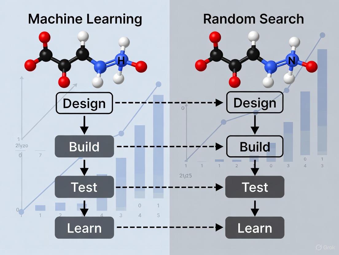
The integration of machine learning into DBTL cycles represents a paradigm shift in metabolic engineering strategy. Traditionally, strain optimization often relied on random search or design of experiment approaches, which could lead to more iterations and extensive consumption of time, money, and resources [5]. Machine learning offers a more efficient path by leveraging biological datasets to build predictive models and identify non-obvious design patterns.
Machine Learning-Enhanced DBTL
Machine learning transforms the DBTL cycle by enabling data-driven predictions and designs. ML algorithms can process large biological datasets to identify patterns and relationships that are difficult for humans to discern [8]. In protein engineering, sequence-based language models (ESM, ProGen) and structure-based tools (ProteinMPNN, MutCompute) enable zero-shot prediction of beneficial mutations without additional experimental training [3]. For metabolic pathway optimization, ML methods like gradient boosting and random forest have demonstrated strong performance in the low-data regime, showing robustness to training set biases and experimental noise [7].
The emerging "LDBT" paradigm places learning at the beginning of the cycle, leveraging pre-trained models and existing biological knowledge to generate initial designs [3]. This approach can potentially reduce the number of experimental iterations needed to achieve desired performance. ML also enhances the Learn phase by providing more sophisticated analysis of complex datasets, enabling researchers to extract deeper insights from each DBTL cycle [4].
Random Search Approach
Random search methods involve testing variants selected without prior knowledge or predictive modeling. While sometimes effective, this approach often requires screening large libraries to identify improved strains, making it resource-intensive and time-consuming [5]. In combinatorial pathway optimization, where the number of possible genetic configurations grows exponentially, random search becomes increasingly inefficient as design complexity increases [7]. However, random search remains useful when biological understanding is limited or when exploring completely new design spaces without existing data for training ML models.
Table 2: Machine Learning vs. Random Search in DBTL Optimization
| Aspect | Machine Learning Approach | Random Search Approach |
|---|---|---|
| Design Strategy | Predictive modeling using biological data and patterns | Random selection or design of experiment |
| Data Efficiency | Improves with more data; can leverage existing datasets | Does not benefit from prior knowledge |
| Iteration Speed | Faster convergence to optimal designs | Requires more DBTL cycles |
| Best Application | Complex optimization with available training data | Initial exploration of unknown design spaces |
| Limitations | Requires sufficient data; model training complexity | Resource-intensive; limited by screening capacity |
| Performance | Gradient boosting/random forest outperform in low-data regimes [7] | Less efficient as design complexity increases [7] |
Case Study: DBTL-Driven Dopamine Production inE. coli
A recent study demonstrates the application of a knowledge-driven DBTL cycle to optimize dopamine production in Escherichia coli, resulting in significant improvements over previous efforts [5]. This case study illustrates the practical implementation of DBTL principles and provides a comparative framework for evaluating metabolic engineering strategies.
Experimental Protocol and Workflow
The researchers employed a systematic approach to engineer an efficient dopamine production strain:
Host Strain Engineering: The base E. coli strain FUS4.T2 was engineered for enhanced L-tyrosine production by depleting the transcriptional dual regulator TyrR and introducing feedback-resistant mutations in chorismate mutase/prephenate dehydrogenase (TyrA) [5].
Pathway Design: The dopamine biosynthetic pathway was constructed using the native E. coli gene encoding 4-hydroxyphenylacetate 3-monooxygenase (HpaBC) to convert L-tyrosine to L-DOPA, and Pseudomonas putida-derived L-DOPA decarboxylase (Ddc) to catalyze dopamine formation [5].
In Vitro Prototyping: Before in vivo implementation, the researchers conducted cell-free protein synthesis tests using crude cell lysate systems to evaluate different relative enzyme expression levels, identifying potential bottlenecks [5].
RBS Library Construction: Based on in vitro results, the team created a ribosome binding site (RBS) library to fine-tune the expression of hpaBC and ddc genes. The library was generated by modulating the Shine-Dalgarno sequence while maintaining constant flanking regions to minimize secondary structure effects [5].
High-Throughput Screening: Automated cultivation in minimal medium with appropriate antibiotics and inducers was followed by dopamine quantification. The production strain was cultivated in minimal medium containing 20 g/L glucose, 10% 2xTY, phosphate buffer, MOPS, vitamin B6, phenylalanine, and trace elements [5].
Analytical Methods: Dopamine concentrations were measured using HPLC, with biomass determined by optical density measurements at 600 nm (OD600) [5].
Figure 1: Knowledge-Driven DBTL Workflow for Dopamine Production Optimization
Performance Results and Comparison
The implementation of the knowledge-driven DBTL cycle yielded significant improvements in dopamine production:
Table 3: Dopamine Production Performance Comparison
| Strain / Approach | Dopamine Titer (mg/L) | Specific Productivity (mg/g biomass) | Fold Improvement |
|---|---|---|---|
| Previous State-of-the-Art | 27.0 | 5.17 | 1.0x (baseline) |
| DBTL-Optimized Strain | 69.03 ± 1.2 | 34.34 ± 0.59 | 2.6-6.6x |
The DBTL-optimized strain achieved dopamine concentrations of 69.03 ± 1.2 mg/L, equivalent to 34.34 ± 0.59 mg/g biomass [5]. This represents a 2.6-fold improvement in titer and a 6.6-fold improvement in specific productivity compared to previous state-of-the-art production strains [5]. The researchers attributed this success to their knowledge-driven approach, which combined upstream in vitro investigation with high-throughput RBS engineering to efficiently optimize the metabolic pathway.
The Scientist's Toolkit: Essential Research Reagents and Solutions
Successful implementation of DBTL cycles in metabolic engineering requires specific reagents, tools, and platforms. The following table summarizes key solutions used in advanced metabolic engineering studies:
Table 4: Essential Research Reagents and Solutions for DBTL Implementation
| Reagent / Solution | Function | Application Example |
|---|---|---|
| Cell-Free Protein Synthesis Systems | Rapid in vitro prototyping of pathway enzymes without cellular constraints | Testing enzyme expression levels before in vivo implementation [5] |
| Ribosome Binding Site (RBS) Libraries | Fine-tuning translation initiation rates for metabolic pathway balancing | Optimizing relative expression of HpaBC and Ddc in dopamine pathway [5] |
| Automated DNA Assembly Platforms | High-throughput construction of genetic variants | Building large libraries of pathway variants for screening [6] |
| Analytical Chromatography (HPLC) | Precise quantification of target compounds and metabolites | Measuring dopamine production titers in culture supernatants [5] |
| CRISPR-Cas Genome Editing Tools | Precise genomic modifications in host strains | Engineering host metabolism for enhanced precursor supply [5] |
| Machine Learning Algorithms | Predictive modeling of sequence-function relationships | Zero-shot prediction of beneficial protein mutations [3] |
Emerging Trends: ML-Driven DBTL and Future Directions
The integration of machine learning is transforming traditional DBTL cycles into more efficient, predictive workflows. Several emerging trends are shaping the future of DBTL in metabolic engineering:
From DBTL to LDBT: A Paradigm Shift
The conventional DBTL cycle is evolving toward an "LDBT" (Learn-Design-Build-Test) paradigm, where learning precedes design through machine learning and prior knowledge [3]. This approach leverages pre-trained models on large biological datasets to generate initial designs, potentially reducing the number of experimental iterations needed. Protein language models trained on evolutionary relationships (ESM, ProGen) and structure-based design tools (ProteinMPNN) enable zero-shot prediction of beneficial mutations without additional training [3]. As these models improve, they may enable first-pass success in biological design, moving synthetic biology closer to the "Design-Build-Work" model seen in established engineering disciplines [3].
Cell-Free Systems for Accelerated Building and Testing
Cell-free expression platforms are emerging as powerful tools for accelerating the Build and Test phases of DBTL cycles [3]. These systems enable rapid protein synthesis without time-intensive cloning steps, with capabilities to produce >1 g/L protein in <4 hours [3]. When combined with liquid handling robots and microfluidics, cell-free systems allow ultra-high-throughput testing of thousands of variants. For example, DropAI leveraged droplet microfluidics to screen over 100,000 picoliter-scale reactions [3]. These platforms are particularly valuable for generating large training datasets for machine learning models, creating a virtuous cycle of improvement.
Automated Biofoundries and Closed-Loop DBTL
The automation of DBTL cycles through biofoundries represents another significant trend [6] [4]. These facilities integrate robotic systems for DNA assembly, strain cultivation, and performance characterization, dramatically increasing throughput and reproducibility. Automated biofoundries enable systematic exploration of large design spaces that would be impossible with manual methods [6]. Furthermore, closed-loop systems that integrate ML agents with automated experimentation can continuously propose and test new designs without human intervention [3]. As these platforms mature, they will enable more complex metabolic engineering projects with reduced development timelines.
Figure 2: Evolution from Traditional to ML-Enhanced DBTL Cycles
The DBTL framework continues to be a pillar of systematic metabolic engineering, providing a structured approach to biological design that balances rational planning with empirical optimization. The integration of machine learning, automation, and computational modeling is transforming DBTL from a sequential process into an integrated, data-driven workflow with the potential to dramatically accelerate strain development. As these technologies mature, the DBTL cycle will become increasingly predictive and efficient, enabling more sophisticated metabolic engineering projects and expanding the range of products accessible through biotechnology. The continued evolution of the DBTL framework promises to enhance our ability to program biology for sustainable manufacturing, therapeutic applications, and fundamental biological discovery.
Table of Contents
- The Critical Role of Hyperparameters in Machine Learning
- Quantitative Comparison of Tuning Strategies
- Experimental Protocols in Hyperparameter Optimization
- Visualizing Hyperparameter Optimization Workflows
- The Scientist's Toolkit: Research Reagent Solutions
The Critical Role of Hyperparameters in Machine Learning
In the context of Design-Build-Test-Learn (DBTL) cycles for drug development, the "Learn" phase involves refining models to guide the next "Design." Hyperparameter tuning is the cornerstone of this phase, transforming a model from a conceptual framework into a predictive tool with real-world impact. Hyperparameters are the configuration settings that govern the machine learning training process itself, set before learning begins [9] [10]. They are distinct from model parameters, which are learned from the data during training [10].
The necessity of tuning stems from the direct influence hyperparameters have on a model's ability to generalize from training data to unseen validation and test sets, a property paramount for predicting compound efficacy or toxicity. A poorly tuned model is often overfit—it performs well on its training data but fails spectacularly in the real world, a phenomenon described as the "silent killer of ROI" in industrial applications [9]. Conversely, an undertuned model may be underfit, failing to capture essential relationships in the data [10]. Systematic hyperparameter optimization minimizes the loss function, bridging the gap between a "meh" model and one that creates tangible value [9]. This is not merely about squeezing out a few extra points of accuracy; a performance jump from 85% to 94% in a fraud detection model, for instance, represented a 60% reduction in error and saved millions [9]. In drug discovery, such improvements can translate to significantly higher success rates in virtual screening or more accurate toxicity predictions, directly accelerating the DBTL cycle.
Quantitative Comparison of Tuning Strategies
The choice of hyperparameter optimization strategy involves a critical trade-off between computational resources and the performance of the final model. The table below summarizes the key characteristics of three primary tuning methods.
Table 1: Comparison of Hyperparameter Tuning Methods
| Method | Core Principle | Computational Efficiency | Best-Suited Scenario | Key Advantage | Key Disadvantage |
|---|---|---|---|---|---|
| Grid Search [11] [12] [10] | Exhaustively evaluates all combinations in a predefined grid. | Low; becomes infeasible with many parameters ("curse of dimensionality"). | Small, well-understood search spaces with few hyperparameters. | Guaranteed to find the best combination within the defined grid. | Computationally expensive and slow, especially with a large number of hyperparameters. |
| Random Search [11] [12] [10] | Randomly samples a fixed number of combinations from defined distributions. | Medium; does not suffer from the curse of dimensionality. | Larger search spaces where some parameters are more important than others. | Often finds good configurations faster than Grid Search; more efficient for a large number of hyperparameters. | Not guaranteed to find the optimal combination; can miss the best hyperparameters. |
| Bayesian Optimization [9] [13] [10] | Builds a probabilistic model to predict promising hyperparameters based on past results. | High; aims to find excellent configurations with far fewer iterations. | Expensive-to-train models (e.g., deep learning) with large, complex search spaces. | Highly sample-efficient; intelligently balances exploration and exploitation. | Sequential nature can lead to longer wall-clock time; more complex to implement. |
Table 2: Illustrative Performance Data on a Wine Quality Dataset [12]
| Tuning Method | Sampled Hyperparameters | Best Accuracy | Computational Note |
|---|---|---|---|
| Grid Search | Exhaustive search over 216 combinations (max_depth: [3,5,10,None], n_estimators: [10,100,200], etc.) |
0.74 | Evaluates all combinations, which is computationally intensive. |
| Random Search | 500 iterations sampled from broader distributions (e.g., n_estimators: 10 to 500) |
0.74 | Achieved comparable accuracy to Grid Search with a more efficient search. |
The data in Table 2 highlights a key insight: Random Search can achieve performance on par with Grid Search but with significantly greater efficiency, as it does not waste resources on unpromising regions of the search space [11]. For the most computationally intensive models in deep learning, Bayesian Optimization is the state-of-the-art method, capable of slashing search time by 10x or more by using a model to guide the search [9].
Experimental Protocols in Hyperparameter Optimization
A rigorous and reproducible experimental protocol is non-negotiable for reliable hyperparameter tuning. The following methodology is standard practice and should be integrated into the DBTL workflow.
1. Data Partitioning: The dataset is first split into training, validation, and hold-out test sets. The training set is used to learn model parameters for each hyperparameter configuration. The validation set is used to evaluate and compare the performance of these different hyperparameter configurations. The test set is used only once, at the very end, to provide an unbiased estimate of the final model's generalization error [14].
2. Defining the Search Space: The researcher must define the hyperparameters to tune and their range of values. This can be a discrete list for Grid Search (e.g., learning_rate: [0.001, 0.01, 0.1]) or a statistical distribution for Random and Bayesian search (e.g., learning_rate: loguniform(1e-5, 1e-2)) [11] [13].
3. Cross-Validation: To mitigate overfitting and provide a more robust performance estimate, k-fold cross-validation is typically employed on the training set. The training data is split into k folds (e.g., 5); the model is trained on k-1 folds and validated on the remaining fold. This process is repeated k times, and the average validation performance is used to score the hyperparameter set [11] [14].
4. Execution and Evaluation: The chosen search algorithm (Grid, Random, or Bayesian) is executed. This involves training and validating a model for each candidate hyperparameter set. The set achieving the best average validation score is selected as the winner.
5. Final Assessment: The final model is retrained on the entire training and validation dataset using the optimal hyperparameters. Its performance is then evaluated on the held-out test set to report the final, unbiased performance metric [14].
Visualizing Hyperparameter Optimization Workflows
The following diagrams illustrate the logical relationships and workflows for the general tuning process and the specific strategies discussed.
General Hyperparameter Tuning Workflow
Comparison of Tuning Strategy Principles
The Scientist's Toolkit: Research Reagent Solutions
Successfully implementing hyperparameter tuning requires a suite of software tools and libraries. The table below details essential "research reagents" for your computational experiments.
Table 3: Essential Software Tools for Hyperparameter Tuning
| Tool / Library | Primary Function | Application in Tuning |
|---|---|---|
| Scikit-learn [11] [14] | A core machine learning library for Python. | Provides the GridSearchCV and RandomizedSearchCV classes for easy implementation of these methods with built-in cross-validation. |
| Optuna [9] | A dedicated hyperparameter optimization framework. | Enables efficient Bayesian optimization with advanced features like pruning (early stopping of poorly performing trials) for complex models like neural networks. |
| Hyperopt [15] | A Python library for serial and parallel optimization. | Similar to Optuna, it allows for Bayesian optimization over complex search spaces for deep learning and other demanding tasks. |
| Cross-Validation [11] [14] | A statistical resampling technique. | Not a software tool per se, but a critical methodological component integrated into tuning workflows to prevent overfitting and ensure robust parameter selection. |
The pharmaceutical industry is undergoing a profound transformation, driven by the integration of artificial intelligence (AI) and machine learning (ML). This shift addresses a critical challenge known as "Eroom's Law"—the paradoxical decline in R&D efficiency despite technological advancements, where the cost of developing a new drug now exceeds $2.23 billion and the process can take 10-15 years with a failure rate of approximately 90% [16]. The traditional drug discovery pipeline, a linear and sequential process of design, build, test, and learn (DBTL), is being superseded by a new, data-driven paradigm. Machine learning algorithms can now parse vast biological and chemical datasets to identify patterns, predict outcomes, and generate novel hypotheses at a scale and complexity beyond human cognition, effectively shifting the center of gravity from the wet lab to the computer—from in vitro to in silico [16].
This overview explores the role of machine learning in drug discovery, framed within a broader thesis on its performance compared to traditional optimization methods like random search within DBTL cycles. By examining experimental data, protocols, and specific case studies, we will demonstrate how ML is not merely accelerating existing processes but is fundamentally recoding the future of pharmaceutical research [16].
Machine Learning vs. Random Search in DBTL Optimization
The classic Design-Build-Test-Learn (DBTL) cycle is the fundamental framework for systematic engineering in synthetic biology and drug discovery. Recently, a paradigm shift has been proposed: LDBT, where "Learning" precedes "Design" [17]. This is made possible by machine learning models that have been pre-trained on massive biological datasets, enabling them to make informed, "zero-shot" predictions to guide the initial design phase [17].
A core research question is how ML-guided learning compares to simpler optimization methods like random search. The key differentiator is that random search explores a design space blindly, whereas ML models learn from iteratively acquired data to predict promising candidates, balancing exploration of unknown regions with exploitation of known high-performing areas [18].
Table: Core Comparison of ML-Guided vs. Random Search Optimization
| Feature | Machine Learning-Guided | Random Search |
|---|---|---|
| Approach | Active learning; predictive models guide next experiments | Passive; random selection from predefined space |
| Data Usage | Learns from cumulative data to refine hypotheses | Ignores data from previous iterations |
| Efficiency | Higher; focuses resources on high-probability candidates | Lower; success is proportional to library size |
| Best For | Complex, high-dimensional optimization problems | Simple problems or establishing a baseline performance |
The implementation of these cycles has been accelerated by technologies like cell-free expression systems for rapid testing and robotic platforms for automation. These platforms can execute fully autonomous "test-learn" cycles, where software analyzes data and directly schedules the next round of experiments without human intervention [17] [18].
Experimental Comparison: A Case Study in Metabolic Engineering
A 2024 study on optimizing p-Coumaric Acid (pCA) production in Saccharomyces cerevisiae provides a clear experimental comparison of ML-guided and random search strategies within a DBTL cycle [19].
Experimental Protocol and Workflow
- Objective: To improve the titer and yield of pCA, a valuable aromatic compound.
- Strain Engineering: Combinatorial libraries were built in yeast, focusing on a 7-gene cluster. Libraries were created by varying both the coding sequences (e.g., feedback-resistant enzyme variants) and regulatory elements (promoters) for key genes in the prephenate pathway [19].
- Library Generation: A one-pot library generation method was used to create diverse strain variants.
- Screening & Data Collection: A subset of the library was screened for pCA production. The resulting genotype-phenotype data was used to train machine learning models.
- ML Model Training: The trained models used feature importance and SHAP (Shapley Additive exPlanations) values to identify which genetic factors most influenced production [19].
- Next-Cycle Design: The ML predictions were used to design a second, optimized library for a subsequent DBTL cycle.
The workflow for this approach is outlined below.
Key Findings and Performance Data
The study demonstrated the superior efficiency of the ML-guided approach. In the first DBTL cycle, which established a baseline, the best-producing strain from the PAL pathway achieved a pCA titer of 0.31 g/L. The ML model, trained on this initial data, was then used to predict a new set of genetic combinations likely to yield higher production [19].
The results from the second DBTL cycle confirmed the model's accuracy. The best strain from this ML-informed library achieved a final pCA titer of 0.52 g/L, representing a 68% increase in production over the first cycle [19]. This direct comparison within a single study provides compelling evidence for the power of ML in pathway optimization.
Table: Performance Outcomes from pCA Optimization DBTL Cycles [19]
| DBTL Cycle | Guidance Strategy | Best pCA Titer (g/L) | Yield on Glucose (g/g) | Key Takeaway |
|---|---|---|---|---|
| Cycle 1 | Initial library screening | 0.31 | Not Specified | Establishes baseline performance and training data. |
| Cycle 2 | Machine Learning prediction | 0.52 | 0.03 | 68% improvement in titer, demonstrating ML efficacy. |
Broader Applications of ML in the Drug Discovery Pipeline
The success of ML in metabolic engineering is mirrored across the entire drug discovery value chain. The following applications highlight its transformative impact.
Target Identification and Validation
ML algorithms analyze complex biological data from genomics, proteomics, and disease pathways to identify and prioritize novel drug targets [20]. For example, Insilico Medicine leveraged AI to identify a novel target for fibrosis in a matter of months, a process that traditionally takes years [20]. Tools like CLAPE-SMB predict protein-DNA binding sites using only sequence data, accelerating this critical first step [21].
Compound Screening and Optimization
AI enables virtual screening of millions of compounds in silico, dramatically outperforming the physical throughput of traditional high-throughput screening (HTS) [22] [20]. Once a "hit" is identified, ML guides the "hit-to-lead" optimization. In a 2025 study, deep graph networks were used to generate over 26,000 virtual analogs, leading to sub-nanomolar inhibitors with a >4,500-fold potency improvement over the initial hit [22]. Predictive models for ADMET (Absorption, Distribution, Metabolism, Excretion, and Toxicity) properties, such as AttenhERG for cardiotoxicity, are also crucial for early risk assessment [21].
Clinical Trial Acceleration
ML streamlines clinical development by optimizing patient recruitment through the analysis of electronic health records, predicting patient response, and reducing dropout rates [23] [20]. It also enables smarter trial design by running virtual scenarios and facilitates real-time monitoring of trial data for early detection of safety signals [20].
The Frontier: Generative AI and Virtual Humans
The field is advancing beyond predictive models to generative AI. Platforms like GALILEO can generate entirely novel drug candidates from scratch. In a 2025 study, GALILEO designed 12 antiviral compounds, achieving a 100% hit rate in subsequent in vitro validation [24]. Looking further ahead, researchers are proposing the development of a "programmable virtual human," an AI-driven systemic model that predicts how a new drug affects the entire human body, not just an isolated target, potentially revolutionizing preclinical safety and efficacy testing [25].
The Scientist's Toolkit: Essential Research Reagents and Platforms
The implementation of ML-driven drug discovery relies on a suite of specialized reagents, software, and hardware.
Table: Key Research Reagent Solutions for ML-Driven Drug Discovery
| Tool Name / Category | Type | Primary Function | Example Use Case |
|---|---|---|---|
| Cell-Free Expression Systems | Wet-lab Reagent Platform | Rapid in vitro protein synthesis and testing without cloning. | Megascale data generation for training ML models; testing protein variants [17]. |
| CETSA (Cellular Thermal Shift Assay) | Wet-lab Assay | Validates direct drug-target engagement in intact cells/tissues. | Providing quantitative, system-level validation of mechanism of action [22]. |
| Protein Language Models (e.g., ESM, ProGen) | Software / Algorithm | Predicts protein structure and function from sequence; designs novel proteins. | Zero-shot prediction of beneficial mutations and antibody sequences [17]. |
| Structure-Based Design Tools (e.g., ProteinMPNN) | Software / Algorithm | Designs new protein sequences that fold into a given backbone structure. | Engineering TEV protease variants with improved catalytic activity [17]. |
| Automated Robotic Platforms | Hardware / Platform | Executes liquid handling, cultivation, and measurement fully autonomously. | Running closed-loop, autonomous DBTL cycles without human intervention [18]. |
| ADMET Prediction Tools (e.g., AttenhERG, Stability Oracle) | Software / Algorithm | Predicts pharmacokinetics, toxicity, and stability of molecules in silico. | Early identification of compounds with hERG liability or poor solubility [17] [21]. |
Machine learning is fundamentally recoding the drug discovery process, moving it from a realm reliant on serendipity and brute-force screening to one driven by predictive, data-driven intelligence. The experimental evidence, particularly from direct comparisons within DBTL cycles, clearly demonstrates that ML-guided optimization outperforms traditional methods like random search in efficiency and outcomes, as shown by the significant increase in product titers in metabolic engineering case studies [19]. The proliferation of ML applications—from target identification and virtual screening to generative AI and autonomous robotic platforms—underscores its role as the central nervous system of modern pharmaceutical R&D [23]. While challenges in data quality, model interpretability, and regulatory acceptance remain, the paradigm has irrevocably shifted. The future of drug discovery lies in the continued integration and refinement of these intelligent systems, promising to deliver life-saving therapies to patients faster and more efficiently than ever before.
In the high-stakes field of drug development, where attrition rates are staggering and development cycles regularly span 10-15 years, efficiency in every process is paramount [26]. The emerging paradigm of Model-Informed Drug Development (MIDD) leverages quantitative approaches to streamline discovery and reduce costly late-stage failures [27]. Within this framework, machine learning (ML) models have become indispensable tools, from predicting drug-target interactions to optimizing clinical trial designs. However, the performance of these ML models hinges critically on their hyperparameter configurations—the settings that govern the learning process itself. The process of identifying these optimal configurations, known as hyperparameter optimization, represents a significant computational challenge. This article examines two fundamental approaches to this challenge—Grid Search and Random Search—within the context of drug development research. We demonstrate how Random Search provides a computationally efficient alternative to Grid Search, enabling researchers to extract maximum predictive power from their models while conserving valuable computational resources that can be redirected toward other critical aspects of the drug development pipeline.
Hyperparameter Fundamentals: Parameters vs. Hyperparameters
In machine learning, a critical distinction exists between model parameters and hyperparameters. Parameters are the internal variables of a model that are learned directly from the training data, such as weight coefficients in linear regression or connection weights in neural networks [28]. These values are optimized during the training process and are not set manually by the researcher. In contrast, hyperparameters are external configuration variables that govern the overall learning process. They are set before the training begins and control aspects such as model capacity, learning speed, and regularization strength [28].
Key Hyperparameters in Machine Learning Algorithms
- Random Forest: nestimators (number of trees), maxdepth (maximum tree depth), minsamplessplit (minimum samples required to split a node) [28]
- Support Vector Machines: C (regularization parameter), kernel (kernel function type), gamma (kernel coefficient) [28] [29]
- Neural Networks: learningrate (step size in gradient descent), batchsize (number of samples per gradient update), hiddenlayercount (number of hidden layers) [28]
- XGBoost: learningrate, nestimators, maxdepth, minchild_weight, subsample [29]
The primary goal of hyperparameter optimization is to identify configurations that provide the optimal balance between overfitting and underfitting, thereby maximizing a model's generalization performance on unseen data [28]. Empirical studies show that hyperparameter selection can have as much impact on model performance as parameter optimization itself, making systematic hyperparameter optimization methodologies essential for developing robust machine learning models [28].
Grid Search: The Systematic Approach
Principles and Methodology
Grid Search represents the most exhaustive and systematic approach to hyperparameter optimization. This method operates on a simple but computationally intensive principle: it performs an exhaustive search across a predefined set of hyperparameter values, evaluating every possible combination [28] [30]. The algorithm follows four key steps: (1) parameter space definition, where discrete value sets are specified for each hyperparameter; (2) Cartesian product calculation, which systematically generates all parameter combinations; (3) model evaluation, where each combination is assessed using cross-validation methodology; and (4) optimal configuration selection, where the parameter set with the highest validation score is chosen [28].
Table 1: Grid Search Workflow Example for SVM Tuning
| Step | Action | Example for SVM |
|---|---|---|
| 1. Define Grid | Specify discrete values for each hyperparameter | C: [0.1, 1, 10, 100], gamma: [1, 0.1, 0.01, 0.001], kernel: ['rbf', 'poly'] |
| 2. Generate Combinations | Create Cartesian product of all values | 4×4×2 = 32 unique combinations |
| 3. Evaluate Models | Train and validate each combination | 5-fold cross-validation = 32×5 = 160 model fits |
| 4. Select Best | Choose configuration with highest performance | Best parameters and score returned |
Advantages and Limitations
Grid Search's primary strength lies in its comprehensive nature—it guarantees finding the global optimum within the defined discrete parameter space, provided the optimal configuration exists within the grid [28] [30]. This deterministic nature produces reproducible results, which is valuable in regulated environments like pharmaceutical research. Additionally, the method is embarrassingly parallelizable, as each parameter combination can be evaluated independently [28].
However, Grid Search contains significant disadvantages in terms of computational complexity. The total number of evaluations grows exponentially with the number of parameters (d) and the number of values per parameter (n), following O(n^d) [28]. This "curse of dimensionality" makes the method impractical for high-dimensional parameter spaces. Furthermore, Grid Search requires sub-optimization in continuous parameter spaces due to its discrete value limitation and can waste computational resources on insignificant parameters [28].
Random Search: The Efficient Alternative
Principles and Methodology
Random Search, proposed by Bergstra and Bengio (2012) as an empirical solution to Grid Search's computational costs, introduces a probabilistic approach to hyperparameter optimization [28]. Instead of exhaustively exploring a predefined grid, Random Search performs the search by randomly sampling parameter combinations from predefined probability distributions [28] [30]. The algorithm follows these steps: (1) parameter distribution definition, where probability distributions are specified for each hyperparameter; (2) sampling strategy, where random combinations are generated according to the n_iter parameter; (3) performance evaluation, where model performance is measured for each sample combination using cross-validation; and (4) optimum selection, where the parameter set with the highest validation score is chosen [28].
Table 2: Random Search Workflow Example for SVM Tuning
| Step | Action | Example for SVM |
|---|---|---|
| 1. Define Distributions | Specify probability distributions for each hyperparameter | C: loguniform(0.1, 100), gamma: loguniform(0.001, 1), kernel: ['rbf', 'poly'] |
| 2. Sample Combinations | Randomly select n_iter parameter sets | n_iter = 20 → 20 unique combinations |
| 3. Evaluate Models | Train and validate each combination | 5-fold cross-validation = 20×5 = 100 model fits |
| 4. Select Best | Choose configuration with highest performance | Best parameters and score returned |
Theoretical Advantages
Random Search's effectiveness stems from the heterogeneous distribution of parameter effects in most machine learning models [28]. In practice, performance is typically determined by a few critical parameters, while others show marginal effects. Random Search benefits from the fact that it does not waste evaluations on exhaustively exploring unimportant parameters, unlike Grid Search which expends equal resources on all dimensions [28]. Mathematically, if the parameter space is d-dimensional and the optimal region lies in a d-subspace, Random Search's probability of discovering the optimal region is generally higher than Grid Search for a fixed computational budget [28].
Direct Comparison: Grid Search vs. Random Search
Computational Efficiency
Random Search demonstrates superior computational efficiency compared to Grid Search, particularly in high-dimensional spaces. In a practical experiment tuning a Random Forest classifier, Grid Search evaluated 648 parameter combinations with 3-fold cross-validation, resulting in 1,944 total model fits [30]. The best score achieved was 0.9648, with a test accuracy of 0.9649 [30]. In contrast, Random Search can achieve competitive performance with significantly fewer evaluations. For instance, in another experiment, Random Search found effective hyperparameters with just 30 samples, requiring only 150 model fits with 5-fold cross-validation—dramatically reducing computation time while maintaining performance [31].
Table 3: Performance Comparison of Grid Search vs. Random Search
| Metric | Grid Search | Random Search |
|---|---|---|
| Search Pattern | Exhaustive, systematic | Random sampling from distributions |
| Parameter Space | Discrete, predefined values | Continuous and discrete distributions |
| Computational Cost | Exponential O(n^d) | Linear O(n) |
| Best for | Small parameter spaces (1-3 dimensions) | High-dimensional spaces (4+ dimensions) |
| Optimal Solution | Guaranteed within grid | Probabilistic, not guaranteed |
| Parallelizability | Excellent (embarrassingly parallel) | Excellent (embarrassingly parallel) |
| Key Advantage | Comprehensive coverage | Broad exploration with fixed budget |
Practical Performance
Empirical evidence consistently shows that Random Search can find equal or better hyperparameter configurations with significantly fewer computational resources. In a case study using the Wine dataset and SVM model tuning, Random Search outperformed Grid Search in accuracy, achieving a score of 0.7569 compared to Grid Search's 0.7459 [32]. This performance advantage arises because Random Search can explore a broader range of values for each hyperparameter, rather than being restricted to a fixed grid [32]. This flexibility is particularly valuable when the relationships between hyperparameters and objective functions are unknown or complex, which is often the case in drug discovery applications involving high-dimensional biological data [32].
Experimental Protocols and Implementation
Standard Implementation Code
Implementing Random Search is straightforward using popular machine learning libraries. The following code example demonstrates Random Search implementation using scikit-learn's RandomizedSearchCV:
This code example showcases random search using scikit-learn's RandomizedSearchCV [31]. Instead of fixed lists, probability distributions enable continuous and flexible exploration of the parameter space. Rather than evaluating thousands of combinations as in a traditional grid search, sampling just 30 dramatically reduces computation while still finding competitive solutions [31].
Experimental Workflow Visualization
The following diagram illustrates the logical workflow of a Random Search optimization process for hyperparameter tuning:
Research Reagent Solutions: Essential Tools for Optimization Experiments
Table 4: Essential Research Tools for Hyperparameter Optimization
| Tool/Category | Specific Examples | Function in Research |
|---|---|---|
| Programming Languages | Python, R | Core implementation languages for optimization algorithms |
| Machine Learning Libraries | scikit-learn, XGBoost, TensorFlow, PyTorch | Provide implemented ML models and tuning capabilities |
| Hyperparameter Optimization Frameworks | Scikit-learn's RandomizedSearchCV, GridSearchCV | Implement standard tuning methods with cross-validation |
| Probability Distributions | scipy.stats (randint, uniform, loguniform) | Define parameter search spaces for random sampling |
| Visualization Tools | Matplotlib, Seaborn, Plotly | Analyze and present optimization results |
| Computational Resources | Multi-core CPUs, Cloud computing platforms | Enable parallel evaluation of parameter configurations |
Advanced Optimization Techniques
Beyond Random Search: Bayesian Optimization
While Random Search represents a significant improvement over Grid Search, more advanced techniques like Bayesian Optimization can provide further efficiencies. Bayesian optimization uses a probabilistic model to approximate the relationship between hyperparameters and model performance, focusing sampling on regions more likely to contain optimal values [31] [29]. This approach is particularly valuable when computational resources are limited and each evaluation is expensive. Studies have shown Bayesian optimization can find optimal hyperparameters in as few as 67 iterations, outperforming both Grid and Random Search methods in terms of efficiency [29].
Quasi-Random Search
Another advanced approach is Quasi-random Search, based on low-discrepancy sequences. This method can be thought of as "jittered, shuffled grid search" that uniformly but randomly explores a given search space, spreading out search points more effectively than pure random search [33]. The advantages include consistent and statistically reproducible behavior, non-adaptive sampling that enables flexible post hoc analysis, and better performance in high-parallelism environments where many trials run simultaneously [33].
Applications in Drug Development and Research
In pharmaceutical research, efficient hyperparameter optimization directly translates to reduced computational costs and accelerated model development. For example, in drug classification and target identification tasks—critical yet challenging steps in drug discovery—properly tuned models can achieve accuracy exceeding 95% [34]. The proposed optSAE + HSAPSO framework integrates a stacked autoencoder for robust feature extraction with a hierarchically self-adaptive particle swarm optimization algorithm for parameter optimization, demonstrating how advanced optimization techniques can enhance pharmaceutical research outcomes [34].
The efficiency of Random Search becomes particularly valuable in drug development contexts where computational resources are often allocated across multiple parallel research efforts. By reducing the time and resources required for model optimization, researchers can iterate more quickly, test more hypotheses, and ultimately accelerate the drug discovery process. This aligns with the broader industry trend toward Model-Informed Drug Development (MIDD), which uses quantitative approaches to improve decision-making across all stages of drug development [27].
Random Search represents a fundamentally more efficient approach to hyperparameter optimization compared to Grid Search, particularly in the high-dimensional parameter spaces commonly encountered in drug discovery research. Its ability to explore broader parameter ranges with fixed computational budget, coupled with its simplicity and excellent parallelization capabilities, makes it particularly suitable for resource-constrained research environments. While advanced techniques like Bayesian optimization offer further refinements, Random Search remains an essential tool in the machine learning practitioner's toolkit—striking an effective balance between implementation complexity and computational efficiency. As drug development increasingly relies on complex machine learning models for tasks ranging from target identification to clinical trial optimization, efficient hyperparameter tuning methods like Random Search will play an increasingly important role in accelerating pharmaceutical research and development timelines.
For years, synthetic biology and bioengineering have been governed by the Design-Build-Test-Learn (DBTL) cycle, an iterative framework that, while systematic, often relies on time-consuming and costly empirical experimentation. The emergence of sophisticated machine learning (ML) and artificial intelligence (AI) is fundamentally challenging this paradigm. A transformative shift is underway, recasting the traditional cycle into a Learn-Design-Build-Test (LDBT) framework. This new paradigm leverages powerful computational models to learn from vast biological datasets before any physical design begins, promising to dramatically accelerate the development of new biological parts, pathways, and therapeutics.
This guide objectively compares the performance of the established DBTL cycle against the emerging LDBT framework, situating the analysis within the broader research context of machine learning versus traditional search and optimization methods, such as random search, in biological engineering.
Understanding the Paradigms: DBTL vs. LDBT
The core difference between the two frameworks lies in the starting point and the role of computational prediction.
The Traditional DBTL Cycle
The conventional Design-Build-Test-Learn (DBTL) cycle is an iterative process [17]:
- Design: Researchers define objectives and design biological constructs (e.g., DNA sequences, proteins) based on domain knowledge and existing models.
- Build: The designed constructs are synthesized and assembled in a biological system (e.g., bacteria, yeast) or in a cell-free environment.
- Test: The performance of the built constructs is experimentally measured (e.g., protein expression, enzyme activity).
- Learn: Data from the test phase are analyzed to inform the next round of design, and the cycle repeats until the desired function is achieved.
This process is inherently empirical and can require multiple lengthy and resource-intensive cycles to converge on a successful solution [17].
The Emerging LDBT Paradigm
The Learn-Design-Build-Test (LDBT) framework represents a fundamental reordering, placing learning at the forefront [17] [35]:
- Learn: The process begins with machine learning models that have been pre-trained on massive biological datasets (e.g., millions of protein sequences, structures, and functional data). These models learn the complex relationships between sequence, structure, and function.
- Design: The trained ML models are used to generate and design new biological constructs with a high probability of success, often through "zero-shot" predictions that do not require additional experimental training data.
- Build & Test: The top-predicted designs are then physically built and tested, often using rapid, high-throughput platforms like cell-free systems.
This approach leverages prior knowledge embedded in ML models to make highly informed initial designs, potentially reducing or eliminating the need for multiple iterative cycles [17].
The following diagram illustrates the fundamental structural differences between these two engineering workflows.
Performance Comparison: LDBT vs. DBTL
The transition from DBTL to LDBT is driven by demonstrated improvements in key performance metrics. The table below summarizes a quantitative comparison based on recent research.
Table 1: Quantitative Performance Comparison of DBTL vs. LDBT Frameworks
| Performance Metric | Traditional DBTL | LDBT Framework | Context & Experimental Evidence |
|---|---|---|---|
| Design Cycles to Candidate | Often requires multiple cycles [17] | Single-cycle success demonstrated [17] | LDBT aims for "single cycle" functional parts via zero-shot prediction [17]. |
| Compounds Synthesized | Thousands to tens of thousands [36] | Hundreds or fewer [36] | Exscientia's AI-designed CDK7 inhibitor required only 136 synthesized compounds [36]. |
| Hit Rate | Low (typical of HTS) | Very High (up to 100% reported) | Model Medicines' GALILEO AI platform achieved a 100% hit rate (12/12 compounds) in antiviral assays [24]. |
| Timeline (Discovery to Candidate) | ~5 years (traditional pharma) [36] | <2 years demonstrated [36] | Insilico Medicine's IPF drug progressed from target to Phase I trials in 18 months [36]. |
| Primary Search Method | Empirical iteration, random/mutagenic sampling [17] | Intelligent navigation of design space [35] | ML uses active learning to select the most informative variants, maximizing information gain per experiment [35]. |
Experimental Protocols & Key Methodologies
The superior performance of the LDBT framework is enabled by specific, advanced methodologies at each stage.
Core LDBT Workflow Protocol
A typical LDBT workflow for a protein engineering campaign involves the following detailed steps:
Learn Phase (Model Training & Foundation):
- Objective: Create a model that maps genetic or protein sequences to functional outputs.
- Procedure: a. Data Curation: Gather a large-scale dataset for training. This can include public databases (e.g., UniProt for sequences, PDB for structures) or proprietary experimental data. b. Model Selection: Choose an appropriate ML architecture. Common choices include: * Protein Language Models (pLMs) like ESM-2 or ProGen, trained on evolutionary sequence data to predict structure and function [17]. * Structure-based Models like ProteinMPNN (for sequence design given a backbone) or AlphaFold2 (for structure prediction) [17]. * Hybrid Physics-Informed ML that incorporates biophysical principles into the model [17]. c. Training: Train the model on the curated dataset to learn the underlying sequence-function relationships.
Design Phase (AI-Driven Generation):
- Objective: Generate novel sequences predicted to have the desired function.
- Procedure: a. In Silico Generation: Use the trained model for zero-shot generation of thousands to billions of candidate sequences. For example, ProGen can generate novel protein sequences conditioned on specific desired properties [17]. b. In Silico Screening: Filter the generated library using predictive models for specific properties like solubility (e.g., with DeepSol), stability (e.g., with Stability Oracle), or target binding (e.g., with molecular docking) [17] [22]. c. Selection: A small set of top-ranking candidates (often tens to hundreds) is selected for experimental validation.
Build Phase (Rapid Synthesis):
Test Phase (High-Throughput Validation):
- Objective: Experimentally measure the function of the built candidates.
- Procedure: Conduct high-throughput assays in line with the target function (e.g., enzyme activity assays, binding assays). Cell-free systems are often coupled directly with robotic liquid handlers and microfluidics (e.g., DropAI platform) to screen >100,000 reactions simultaneously [17].
This integrated workflow is depicted in the following diagram, showing the flow of information and materials between the computational and physical experimental stages.
Case Study: Antimicrobial Peptide Design
A 2025 study exemplifies the power of the LDBT paradigm [17]:
- Learn: Researchers trained deep learning models on datasets of known antimicrobial peptides (AMPs).
- Design: The model computationally surveyed over 500,000 potential AMPs and selected 500 optimal variants for experimental testing.
- Build & Test: The 500 candidates were synthesized and tested.
- Result: The LDBT process identified 6 promising AMP designs with high accuracy, demonstrating efficient navigation of a vast design space that would be prohibitively expensive to explore empirically.
The Scientist's Toolkit: Essential Research Reagents & Platforms
Implementing a robust LDBT pipeline requires a suite of specialized computational and experimental tools.
Table 2: Essential Research Reagents and Platforms for LDBT
| Category | Item / Platform | Function in LDBT Workflow |
|---|---|---|
| Computational Models | Protein Language Models (e.g., ESM, ProGen) [17] | Learn from evolutionary data to predict protein structure and function; enable zero-shot design. |
| Structure-based Design Tools (e.g., ProteinMPNN, RosettaFold) [17] | Design protein sequences that fold into a specific backbone structure. | |
| Property Predictors (e.g., DeepSol, Stability Oracle) [17] | Predict key biophysical properties like solubility and thermodynamic stability from sequence. | |
| Rapid Build/Test Systems | Cell-Free Transcription-Translation (TX-TL) Systems [17] [35] | Rapidly express proteins without live cells, enabling high-throughput building and testing. |
| Microfluidic/Droplet Platforms (e.g., DropAI) [17] | Allow ultra-high-throughput screening of reactions (e.g., >100,000 picoliter-scale reactions). | |
| Automated Biofoundries [17] | Integrated robotic facilities that automate the Build and Test phases for massive parallelism. |
Context: Machine Learning vs. Random Search in DBTL Optimization
The shift from DBTL to LDBT is, at its core, a shift from relying on empirical search methods to leveraging intelligent, model-guided optimization.
- Random Search in Traditional DBTL: The classic DBTL cycle, especially when exploring uncharted biological space, often functions similarly to a random search. While more structured than pure trial-and-error, its efficiency is limited because each cycle does not necessarily inform the next in a globally optimal way. The learning is often local and heuristic, leading to slow convergence and a high risk of becoming trapped in local optima [17].
- Machine Learning in LDBT: Machine learning, particularly active learning, transforms this process. ML models are trained to understand the complex, high-dimensional landscape of biological sequence space. They can predict which regions of this vast space are most likely to be successful, effectively pruning away unproductive avenues of research before any lab work begins [35]. This represents a move from exploring a landscape in the dark to exploring it with a predictive map.
- Quantitative Advantage: The performance metrics in Table 1, such as the drastic reduction in compounds synthesized and the dramatically increased hit rates, provide concrete evidence of ML's superiority over traditional, more stochastic search methods for navigating biological complexity.
The evidence from cutting-edge research paints a clear picture: the LDBT framework is outperforming the traditional DBTL cycle on critical metrics of efficiency, speed, and success rate. By placing machine learning at the beginning of the workflow, researchers can leverage vast biological knowledge to make smarter initial designs, dramatically reducing the need for costly and time-consuming iterative cycles. While the DBTL cycle remains a valuable and foundational engineering concept, the integration of AI and rapid experimentation platforms in the LDBT paradigm represents the future of bioengineering. This shift enables a more predictive, first-principles approach to biological design, poised to accelerate breakthroughs in drug discovery, enzyme engineering, and synthetic biology.
Implementing ML and Random Search in Drug Discovery DBTL Pipelines
Random Search for Efficient Model Tuning in QSAR and Virtual Screening
In modern drug discovery, Quantitative Structure-Activity Relationship (QSAR) modeling and virtual screening have become indispensable tools for identifying promising therapeutic candidates. The performance of machine learning models in these applications heavily depends on selecting appropriate hyperparameters, which control the learning process itself. While sophisticated optimization algorithms continue to emerge, Random Search remains a surprisingly effective and widely adopted approach for hyperparameter tuning in QSAR workflows, particularly given the computational constraints and structured data characteristics common to cheminformatics problems.
This guide provides an objective comparison of Random Search against competing hyperparameter optimization methods within the context of machine learning-driven QSAR and virtual screening. We present experimental data, detailed protocols, and practical recommendations to help researchers select appropriate tuning strategies for their specific drug discovery pipelines.
Theoretical Foundations of Hyperparameter Optimization Methods
Random Search Fundamentals
Random Search operates by evaluating random combinations of hyperparameters sampled from predefined distributions over the parameter space. Unlike systematic approaches, it doesn't attempt to model the performance landscape but relies on statistical probability to find good configurations. The algorithm's effectiveness stems from the empirical observation that for most machine learning models, a small subset of parameters truly drives performance variance. By testing more distinct values for each parameter across the entire search space, Random Search often discovers high-performing regions more efficiently than methods that exhaustively search limited dimensions [37].
Alternative Optimization Strategies
Several competing approaches offer different trade-offs between computational efficiency and solution quality:
- Grid Search: Systematically explores all combinations of a predefined set of values for each hyperparameter. While thorough, it suffers from the "curse of dimensionality" – computational requirements grow exponentially as parameters increase [38].
- Bayesian Optimization: Builds a probabilistic model of the objective function to direct future sampling toward promising regions. It typically requires fewer evaluations but has higher computational overhead per iteration [38].
- Tree-structured Parzen Estimator (TPE): Models the performance landscape using Gaussian distributions to focus sampling on hyperparameter values that previously yielded good results [38].
- Hyperband: Utilizes an early-stopping strategy to quickly discard underperforming configurations, efficiently allocating computational resources [38].
Comparative Performance Analysis
Experimental Framework and Dataset Characteristics
To objectively evaluate optimization methods, we synthesized data from multiple published studies comparing hyperparameter tuning approaches across various machine learning tasks and dataset types. The table below summarizes key dataset characteristics used in these benchmark studies:
Table 1: Dataset Characteristics in Hyperparameter Optimization Studies
| Dataset Name | Samples | Features | Task Type | ML Algorithms Evaluated |
|---|---|---|---|---|
| Iris Flower | 150 | 4 | Multiclass Classification | K-NN, K-means, Neural Networks, SVM |
| Pima Indians Diabetes | 768 | 8 | Binary Classification | K-NN, K-means, Neural Networks, SVM |
| MNIST Handwritten Digits | 70,000 | 784 | Multiclass Classification | K-NN, K-means, Neural Networks, SVM |
| ChEMBL T. cruzi Inhibitors | 1,183 | 1,804 | Regression | SVM, ANN, Random Forest |
Quantitative Performance Comparison
The following table synthesizes performance metrics across multiple studies comparing Random Search to other optimization methods:
Table 2: Performance Comparison of Hyperparameter Optimization Methods
| Optimization Method | Average Accuracy Gain | Computational Efficiency | Implementation Complexity | Best Suited Scenarios |
|---|---|---|---|---|
| Random Search | Baseline | High | Low | Limited computational resources, High-dimensional parameter spaces |
| Random Search Plus | 5-30% improvement over Random Search [37] | High (10% of RS time for equivalent results) [37] | Medium | All problem types, especially when accuracy prioritizes |
| Grid Search | Comparable to Random Search | Low (exponential complexity) | Low | Very low-dimensional spaces, Exhaustive search required |
| Bayesian Optimization | 0-15% improvement over Random Search | Medium (high per-iteration cost) | High | Expensive function evaluations, Low-dimensional spaces |
| Hyperband | Comparable to Random Search | Very High (early stopping) | Medium | Large-scale neural architectures, Distributed computing |
Case Study: Random Search Plus Enhancement
A 2020 study introduced Random Search Plus, which incorporates hyperparameter space separation to improve upon traditional Random Search. The method works by dividing the search space into regions and allocating trials more strategically. Empirical evaluation demonstrated that this enhancement could:
- Find better hyperparameters than traditional Random Search, improving accuracy by 5-30% on supervised learning tasks [37]
- Achieve equivalent optimization as Random Search in only 10% of the time with appropriate space separation strategies [37]
- Provide more globally optimal solutions compared to the sometimes locally-constrained results of traditional Random Search [37]
Experimental Protocols for Hyperparameter Optimization in QSAR
Standard Random Search Implementation Protocol
For researchers implementing Random Search in QSAR workflows, the following protocol provides a robust starting point:
Define Hyperparameter Space: Specify distributions for each hyperparameter (e.g., uniform, log-uniform) based on theoretical constraints and empirical experience.
Set Iteration Budget: Determine the number of random combinations to evaluate based on computational resources (typically 50-200 iterations).
Configure Cross-Validation: Implement k-fold cross-validation (typically k=5 or 10) to evaluate each hyperparameter combination's performance.
Execute Parallel Trials: Evaluate different hyperparameter combinations concurrently to maximize resource utilization.
Select Optimal Configuration: Identify the hyperparameter set yielding the best cross-validated performance metric (e.g., RMSE, MAE, Pearson R²).
Final Model Training: Train the final model using the optimal hyperparameters on the entire training set.
QSAR-Specific Evaluation Metrics
When applying these methods to QSAR and virtual screening, researchers should select evaluation metrics aligned with their specific objectives:
- For regression models predicting continuous activity values (e.g., pIC50, pKi), use RMSE, MAE, and Pearson Correlation Coefficient [39] [40].
- For classification models in virtual screening, prioritize Positive Predictive Value (PPV) over balanced accuracy when screening ultra-large chemical libraries, as it better reflects hit identification performance in early discovery [41].
Integrated Workflow for QSAR Model Development
The following diagram illustrates the complete QSAR model development workflow, highlighting the role of hyperparameter optimization within the broader context:
Table 3: Essential Tools for QSAR Modeling and Hyperparameter Optimization
| Tool/Resource | Type | Function in QSAR/Hyperparameter Optimization | Example Applications |
|---|---|---|---|
| Scikit-learn | Python Library | Provides ML algorithms and hyperparameter optimization implementations | Implementation of Random Search, Grid Search, and cross-validation [39] |
| PaDEL-Descriptor | Software | Calculates molecular descriptors and fingerprints from chemical structures | Generation of 1,804 molecular descriptors for QSAR modeling [39] |
| ChEMBL Database | Chemical Database | Provides curated bioactivity data for model training | Source of 1,183 T. cruzi inhibitors for anti-Chagas disease modeling [39] |
| Random Forest | ML Algorithm | Ensemble method effective for structured data; robust to hyperparameter choices | Classification of active/inactive compounds in virtual screening [42] |
| Support Vector Machine (SVM) | ML Algorithm | Powerful for nonlinear classification; requires careful hyperparameter tuning | Modeling complex structure-activity relationships with RBF kernel [39] |
| Artificial Neural Networks | ML Algorithm | Flexible function approximators; highly sensitive to architecture hyperparameters | Development of high-performance QSAR models with CDK fingerprints [39] |
Based on our comprehensive analysis of hyperparameter optimization methods in the context of QSAR and virtual screening, we provide the following evidence-based recommendations:
Prioritize Random Search Plus over traditional Random Search for most QSAR applications, as it provides significant accuracy improvements (5-30%) or equivalent performance in substantially less time (up to 90% reduction) [37].
Reserve Grid Search for scenarios with very few hyperparameters (typically ≤3), where exhaustive search remains computationally feasible without compromising project timelines.
Consider Bayesian Optimization when function evaluations are computationally expensive and the hyperparameter space is low-dimensional, despite its higher implementation complexity.
Select evaluation metrics aligned with project goals – particularly for virtual screening, where Positive Predictive Value (PPV) better reflects success in identifying true hits from ultra-large chemical libraries than traditional balanced accuracy [41].
Random Search and its enhanced variants continue to offer compelling performance for hyperparameter optimization in QSAR modeling, balancing computational efficiency with competitive results. As drug discovery increasingly relies on large-scale virtual screening of expansive chemical libraries, efficient model tuning remains essential for accelerating the identification of novel therapeutic candidates.
De Novo Drug Design with Deep Learning and Reinforcement Learning
The integration of artificial intelligence (AI) into drug discovery represents a paradigm shift, offering the potential to significantly reduce the time and cost associated with traditional drug development. De novo drug design, the computational generation of novel drug-like molecules from scratch, has emerged as a particularly promising application of AI. This field leverages deep learning architectures and reinforcement learning (RL) to explore the vast chemical space and design molecules with specific pharmacological properties. Within the broader context of machine learning versus random search for Design-Build-Test-Learn (DBTL) cycle optimization, AI-driven methods demonstrate a fundamental advantage: they use learned chemical knowledge to make informed decisions, moving beyond the stochastic sampling of random search to efficiently navigate complex structure-activity relationships. This guide provides an objective comparison of the performance, methodologies, and applications of state-of-the-art deep learning and reinforcement learning frameworks in de novo drug design.
Comparative Analysis of Methodologies and Performance
The performance of AI-driven de novo design models is evaluated against a multitude of criteria, including the bioactivity, synthesizability, and novelty of the generated molecules, as well as their ability to model complex pharmacological phenomena.
Key Model Architectures and Their Experimental Performance
Table 1: Comparison of Key Deep Learning and RL Frameworks for De Novo Drug Design
| Model/Framework | Core Approach | Key Innovation | Reported Experimental Outcome | Primary Advantage |
|---|---|---|---|---|
| DRAGONFLY [43] | Interactome-based Deep Learning (GTNN + LSTM) | "Zero-shot" learning from a drug-target interactome; no application-specific fine-tuning needed. | Generated potent PPARγ partial agonists; crystal structure confirmed anticipated binding mode. | Integrates both ligand- and structure-based design; outperformed fine-tuned RNNs on synthesizability, novelty, and bioactivity [43]. |
| ACARL [44] | Activity Cliff-Aware Reinforcement Learning | Formulates an Activity Cliff Index (ACI) and uses a contrastive RL loss to prioritize activity cliff compounds. | Surpassed state-of-the-art algorithms in generating high-affinity molecules for multiple protein targets [44]. | Explicitly models critical structure-activity relationship (SAR) discontinuities, which are often overlooked. |
| Diversity-Aware RL [45] | Reinforcement Learning with Intrinsic Motivation | Combines structure- and prediction-based methods to penalize rewards and enhance diversity. | Effectively increased the diversity of the set of generated molecules without sacrificing high rewards [45]. | Prevents the optimization process from becoming stuck in local optima. |
| REINVENT/Reg. MLE [46] | Regularized Maximum Likelihood Estimation (RL) | Keeps the agent's policy close to a pre-trained prior policy while focusing on high-scoring sequences. | Demonstrated good sample efficiency and performance in generating predicted active molecules against DRD2 [46]. | Balances the exploration of novel chemical space with the exploitation of known chemical rules. |
Addressing Critical Challenges in Molecular Generation
A significant challenge in the field is the evaluation of generative models. A large-scale analysis of approximately one billion generated molecules revealed that the size of the generated molecular library is a critical confounder. Common evaluation metrics like the Fréchet ChemNet Distance (FCD) can be misleading if the number of designs is too small, with convergence often requiring over 10,000 designs—a larger number than is typically used in many studies [47]. This underscores the importance of standardized, large-scale evaluation for fair model comparison.
Furthermore, traditional methods struggle with activity cliffs, a phenomenon where small structural changes lead to significant shifts in biological activity. The ACARL framework directly addresses this by identifying activity cliff compounds using a quantitative Activity Cliff Index and dynamically enhancing their impact during RL training through a tailored contrastive loss function [44]. This approach allows the model to focus optimization on high-impact regions of the SAR landscape.
Detailed Experimental Protocols
To ensure reproducibility and provide a clear basis for comparison, this section outlines the standard protocols and workflows used in the cited studies.
General DBTL Workflow for AI-Driven Drug Design
The following diagram illustrates the standard Design-Build-Test-Learn (DBTL) cycle, which is foundational to both ML-guided and random search approaches in enzyme engineering and drug design [48].
The ACARL Framework Workflow
The Activity Cliff-Aware Reinforcement Learning (ACARL) framework introduces a specific methodology for incorporating SAR knowledge into the RL loop [44].
Experimental Protocol for ML-Guided Enzyme Engineering
A representative experimental protocol from a study engineering amide synthetases using a machine-learning guided cell-free platform is detailed below [48]:
- Explore Substrate Promiscuity: Evaluate the wild-type enzyme's (e.g., wt-McbA) activity against a broad panel of potential substrates (e.g., 1100 unique reactions) to identify challenging but desirable chemical transformations.
- Generate Sequence-Function Data:
- Cell-Free DNA Assembly: Use PCR with primers containing nucleotide mismatches to introduce desired mutations, followed by DpnI digestion and Gibson assembly to create mutated plasmids.
- Cell-Free Protein Expression: Amplify linear DNA expression templates (LETs) and express the mutated protein variants using a cell-free gene expression system.
- Functional Assay: Test the expressed enzyme variants for the desired activity (e.g., amide bond formation) under relevant conditions.
- Train Machine Learning Model: Use the collected data (e.g., 1217 enzyme variants tested in 10,953 reactions) to train a supervised ML model, such as an augmented ridge regression model, incorporating an evolutionary zero-shot fitness predictor.
- Predict and Validate: Use the trained model to extrapolate and predict higher-order mutants with increased activity. Synthesize and experimentally validate the top-predicted variants.
The Scientist's Toolkit: Essential Research Reagents and Solutions
Successful implementation of the aforementioned protocols relies on a suite of computational and experimental tools.
Table 2: Key Research Reagents and Solutions for De Novo Drug Design
| Tool/Solution | Type | Primary Function | Application Example |
|---|---|---|---|
| Chemical Language Models (CLMs) [43] [47] | Computational Model | Generates novel molecular structures represented as SMILES or SELFIES strings. | Core generative component in frameworks like DRAGONFLY and in large-scale evaluation studies [43] [47]. |
| Cell-Free Gene Expression (CFE) [48] | Experimental Platform | Rapidly synthesizes and tests proteins without the need for cellular transformation and cloning. | Enabled high-throughput mapping of sequence-function relationships for enzyme variants (1217 variants tested) [48]. |
| Docking Software (e.g., AutoDock, Gnina) [44] [49] | Computational Oracle | Scores protein-ligand binding poses and provides a reward signal (docking score) for RL. | Used in ACARL and other studies to authentically reflect activity cliffs and score generated molecules [44]. |
| Graph Neural Networks (e.g., GTNN, GIN) [43] [49] | Computational Model | Learns from molecular graphs or 3D protein structures to predict properties or generate molecules. | Used in DRAGONFLY to process input graphs and in DeepTGIN to predict binding affinity [43] [49]. |
| Quantitative Structure-Activity Relationship (QSAR) Models [43] | Computational Model | Predicts the bioactivity (e.g., pIC50) of novel molecules based on molecular descriptors. | Used in DRAGONFLY to estimate the on-target bioactivity of de novo designs [43]. |
The comparative analysis presented in this guide demonstrates that deep learning and reinforcement learning frameworks have substantially advanced the field of de novo drug design. Models like DRAGONFLY and ACARL show superior performance over earlier methods by incorporating richer biological context—such as drug-target interactomes and explicit activity cliff modeling—into the generative process. When framed within the broader thesis of ML versus random search for DBTL optimization, the evidence is clear: machine learning approaches, particularly those that are diversity-aware and guided by domain-specific knowledge, provide a more efficient and targeted strategy for navigating the complex fitness landscapes of drug design. They leverage data to make intelligent, iterative decisions, moving far beyond the stochastic sampling of random search. As the field matures, addressing challenges in evaluation standardization and the development of models that better capture the intricacies of biological systems will be key to fully realizing the potential of AI in drug discovery.
Accelerating Build-Test Phases with Cell-Free Systems and High-Throughput Data
The iterative cycle of Design-Build-Test-Learn (DBTL) serves as the fundamental engine of progress in synthetic biology and protein engineering. Within this framework, the Build and Test phases have traditionally constituted significant bottlenecks, often relying on slow, cell-based methods that can take days or weeks. The emergence of sophisticated computational optimization strategies, primarily machine learning (ML)-driven approaches and random search methods, has transformed this paradigm by guiding these biological cycles more intelligently. Concurrently, cell-free protein synthesis (CFPS) systems have emerged as a powerful technological disruptor, offering unprecedented speed and throughput for the Build-Test phases. This guide objectively compares the performance of ML-based and random search DBTL optimization, with a specific focus on how CFPS systems generate the high-throughput data required to fuel these computational models. Framing this comparison is a broader thesis question: under what experimental conditions do the sophisticated predictions of machine learning provide a decisive advantage over the statistical robustness of random search for biological optimization?
The core challenge in DBTL acceleration lies in the efficient exploration of a vast biological design space. Machine learning models, including active learning strategies, aim to reduce the number of experimental iterations by building predictive models from data to inform the next most informative designs. In contrast, random search provides a computationally efficient, statistically grounded baseline by sampling the parameter space without a learned model. The choice between them is not trivial and impacts the speed, cost, and ultimate success of an engineering campaign. As we will demonstrate, the integration of either method with rapid cell-free testing creates a powerful feedback loop, but their relative effectiveness is highly dependent on the specific experimental context, including the dimensionality of the problem and the availability of high-quality data.
Performance Comparison: Machine Learning vs. Random Search
The quantitative comparison between Machine Learning and Random Search reveals a nuanced trade-off between computational efficiency and performance gains. The table below synthesizes experimental data from key studies that have directly compared these optimization strategies in biological contexts.
Table 1: Experimental Comparison of ML and Random Search Performance
| Study Context | Optimization Target | Key Metric | Machine Learning Result | Random Search Result | Reference |
|---|---|---|---|---|---|
| Colicin Protein Production [50] | CFPS yield in E. coli & HeLa systems | Yield Improvement (over baseline) | 2- to 9-fold increase in 4 cycles | Not specifically tested against | [50] |
| Urban Building Energy Modeling (Chicago) [51] | Model Predictive Accuracy (GBDT Algorithm) | R² Score (after tuning) | ~0.840 (Best Achieved) | ~0.827 (Best Achieved) | [51] |
| General Model Tuning [11] | Search Efficiency | Computational Cost | Explores subset of space; more efficient in high dimensions | Explores entire space; computationally expensive | [11] |
| Hyperparameter Optimization [28] | Model Accuracy & Resource Use | Final Performance & Time | Can find near-optimal configs faster | Guaranteed optimum only if in search grid | [28] |
A critical study exemplifies the potential of ML-driven DBTL. Researchers established a fully automated pipeline using an active learning (AL) strategy to optimize cell-free production of the antimicrobial proteins colicin M and E1. This approach achieved a 2- to 9-fold increase in protein yield in just four DBTL cycles [50]. The "Learn" phase employed a cluster margin (CM) sampling strategy, which selects experimental conditions that are both uncertain to the model and diverse from each other, thereby maximizing information gain from each cycle. This result highlights the power of ML to rapidly converge on high-performing solutions with minimal experimental iteration.
In a broader engineering context, a comparative study on urban building energy models (UBEMs) provides a direct performance comparison. When tuning a Gradient Boosted Decision Tree (GBDT) model, both ML-based and random search methods improved performance over default settings. However, the ML-driven tuning narrowly outperformed random search, achieving an R² of approximately 0.840 compared to 0.827 [51]. This suggests that while both methods are effective, ML can extract marginal gains in predictive accuracy.
The primary advantage of random search lies in its computational efficiency, particularly in high-dimensional spaces. As noted in guides on hyperparameter optimization, grid search (a structured exhaustive search) suffers from the "curse of dimensionality," where the number of required experiments grows exponentially with each new parameter [28] [11]. Random search does not have this limitation; it can sample a wider, more effective range of values for each parameter with a fixed experimental budget, often finding good solutions faster than an exhaustive grid search [11].
Experimental Protocols and Workflows
Automated DBTL Workflow for CFPS Optimization
The following protocol details the automated, ML-driven DBTL cycle used to optimize protein yields in CFPS, as demonstrated in the colicin production study [50].
- Phase 1: Design (AI-Driven). The process begins with the formal definition of the optimization goal (e.g., maximizing colicin M yield). The experimental space is defined, typically encompassing factors like DNA template concentration, concentrations of energy sources (e.g., ATP, amino acids), and salt conditions (e.g., Mg²⁺). In the referenced study, a key innovation was the use of ChatGPT-4 to generate all necessary Python code for the experimental design and microplate layout without manual revision, demonstrating the emerging role of LLMs in automating scientific coding [50].
- Phase 2: Build (Automated Setup). A liquid handling robot prepares the CFPS reactions in a microplate format according to the designed layout. The CFPS system itself—whether based on E. coli lysate or HeLa cell lysate—is assembled from a master mix combined with the variable components. This step ensures high reproducibility and eliminates manual errors.
- Phase 3: Test (High-Throughput Analysis). The microplate is incubated to allow for protein synthesis. Protein yield is then quantified using a plate reader, typically by measuring the fluorescence or luminescence of a reporter protein co-expressed with the target or via a direct assay for the target protein. This generates the high-throughput quantitative data that fuels the learning phase.
- Phase 4: Learn (Active Learning Model). The yield data from the Test phase is used to retrain a machine learning model (e.g., a Gaussian process model). The model then uses the Cluster Margin sampling strategy to select the next set of conditions to test. This strategy balances exploration (testing diverse conditions) and exploitation (testing conditions predicted to be high-yielding) by selecting samples that are both uncertain to the model and diverse from each other [50]. This refined batch of experiments is then fed into the next Design phase, closing the loop.
The workflow's logical structure and the specific strategy of the Learning phase can be visualized as follows:
High-Throughput Screening Assay for Drug Discovery
Beyond optimizing protein production, CFPS systems are pivotal in high-throughput screening (HTS) for drug discovery. A relevant protocol is the development of a TR-FRET (Time-Resolved Fluorescence Resonance Energy Transfer) assay to find inhibitors of the SLIT2/ROBO1 protein-protein interaction, a key target in cancer and other diseases [52].
- Step 1: Protein Production. Recombinant SLIT2 and ROBO1 proteins are produced, ideally using a CFPS system to ensure rapid, high-yield, and functional expression of these often-difficult-to-express proteins [53] [54].
- Step 2: Assay Development. The purified proteins are tagged with donor and acceptor fluorophores compatible with TR-FRET. The assay conditions (buffer, protein concentrations, detergent) are optimized to maximize the signal-to-noise ratio of the interaction.
- Step 3: Library Screening. A chemical library of small molecules is dispensed into assay plates using liquid handlers. The SLIT2 and ROBO1 protein mixtures are added to each well, and after incubation, the TR-FRET signal is measured. A loss of signal indicates a disruption of the protein interaction.
- Step 4: Hit Validation. Compounds identified as "hits" from the primary screen are re-tested in dose-response experiments to confirm activity and determine potency (IC50 values). This workflow, from protein production to hit identification, is dramatically accelerated by the use of CFPS, which avoids the weeks-long process of cell-based protein expression [52].
Essential Research Reagent Solutions
The successful implementation of the aforementioned workflows relies on a suite of specialized reagents and materials. The table below details key components for a CFPS-based optimization or screening campaign.
Table 2: Key Reagent Solutions for CFPS and High-Throughput Workflows
| Item | Function | Specific Examples & Notes |
|---|---|---|
| Cell-Free Lysate | Provides the enzymatic machinery for transcription and translation. | Choice depends on target protein; common lysates are from E. coli (cost-effective), wheat germ (high-yield), or mammalian cells like HeLa (complex PTMs) [53] [50]. |
| Energy System | Fuels the protein synthesis reaction by regenerating ATP. | Typically includes phosphoenolpyruvate (PEP) or creatine phosphate and creatine kinase [53]. |
| DNA Template | Encodes the target protein for expression. | Can be a linear PCR product or plasmid; CFPS bypasses cloning, allowing direct use of linear templates [53]. |
| Amino Acid Mixture | Building blocks for protein synthesis. | A mixture of all 20 canonical amino acids is standard. Can be modified with non-canonical amino acids for specific applications [53]. |
| Membrane Mimetics | Solubilizes and stabilizes membrane proteins during synthesis. | Detergents, nanodiscs, or liposomes can be added directly to the CFPS reaction [53] [54]. |
| Fluorescent Reporters | Enables rapid, high-throughput quantification of protein yield or activity. | Used in plate reader assays for real-time monitoring or end-point measurements [50]. |
| Automation Equipment | Enables reproducible, high-throughput setup of reactions. | Liquid handling robots and digital microfluidics (DMF) systems for nanoliter-scale reactions [50] [54]. |
Logical Comparison of Optimization Strategies
The choice between machine learning and random search is not a simple matter of which is "better," but rather which is more suitable for a given problem structure. The following diagram illustrates the logical decision process for selecting an optimization strategy, based on the context of the search space and available resources.
The integration of cell-free systems with high-throughput data collection has irrevocably altered the landscape of the Build-Test phases, providing the empirical fuel for advanced computational optimization. The comparative analysis presented in this guide underscores a critical conclusion: the performance of machine learning versus random search is context-dependent.
For problems characterized by high-dimensional search spaces and where initial data exists to seed a model, machine learning-driven active learning provides a superior strategy. Its ability to intelligently select the most informative experiments leads to faster convergence and higher performance gains, as demonstrated by the multi-fold yield improvements in CFPS [50]. Furthermore, the automation of the Design phase using large language models (LLMs) is set to further lower the barrier to implementing sophisticated ML cycles [50]. However, this approach requires greater computational expertise and infrastructure.
In contrast, random search remains a powerful, robust, and easily implementable alternative. It is particularly effective when dealing with a large number of parameters and when computational efficiency and simplicity are paramount [28] [11]. It avoids the potential pitfalls of a poorly specified ML model and can efficiently explore the parameter space with a fixed experimental budget.
The broader thesis of DBTL optimization research points toward a hybrid future. The paradigm is even shifting from DBTL to "LDBT," where Learning from vast datasets and pre-trained models precedes and informs the initial Design [17]. In this new model, foundational knowledge, whether from biophysical principles or protein language models like ESM and ProGen, is built into the cycle from the start [17]. The choice between advanced ML and random search will therefore be guided by the specific problem, but both will be powerfully accelerated by the open, configurable, and rapid platform provided by cell-free biology.
Drug-Target Interaction (DTI) prediction is a critical task in the drug discovery pipeline, aimed at identifying whether a drug molecule (ligand) interacts with a specific protein target. Accurate DTI prediction can significantly accelerate drug repurposing and reduce the costs associated with experimental validation. Within the broader thesis of machine learning versus random search in Design-Build-Test-Learn (DBTL) optimization research, evaluating algorithm performance is paramount. The DBTL cycle, a cornerstone of synthetic biology and drug discovery, involves designing biological systems, building them, testing their functionality, and learning from the data to inform the next design cycle. Recent proposals even suggest reordering this cycle to "LDBT" (Learn-Design-Build-Test), where machine learning models utilizing large datasets precede and guide the design phase, potentially reducing iterative cycling [17]. Within this optimized framework, selecting the right predictive algorithm for tasks like DTI becomes crucial. This guide objectively compares three key algorithms—Random Forest, Support Vector Machines, and Deep Neural Networks—in the context of DTI prediction, providing experimental data and methodologies to inform researchers and drug development professionals.
Algorithm Performance Comparison
The performance of DTI prediction models is typically evaluated on benchmark datasets like BindingDB, Davis, and KIBA using standard classification metrics. The following table summarizes the quantitative performance of key algorithms as reported in recent studies.
Table 1: Performance Comparison of DTI Prediction Algorithms on Benchmark Datasets
| Algorithm / Model | Dataset | Accuracy (%) | Precision (%) | Recall/Sensitivity (%) | F1-Score (%) | ROC-AUC (%) |
|---|---|---|---|---|---|---|
| Random Forest (RF) [55] | BindingDB-Kd | 97.46 | 97.49 | 97.46 | 97.46 | 99.42 |
| Random Forest (RF) [55] | BindingDB-Ki | 91.69 | 91.74 | 91.69 | 91.69 | 97.32 |
| EviDTI (Deep Learning) [56] | DrugBank | 82.02 | 81.90 | - | 82.09 | - |
| EviDTI (Deep Learning) [56] | Davis | ~0.8% higher than best baseline* | ~0.6% higher than best baseline* | - | ~2% higher than best baseline* | ~0.1% higher than best baseline* |
| EviDTI (Deep Learning) [56] | KIBA | ~0.6% higher than best baseline* | ~0.4% higher than best baseline* | - | ~0.4% higher than best baseline* | ~0.1% higher than best baseline* |
| Support Vector Machine (SVM) [56] | DrugBank | (Competitive baseline) | (Competitive baseline) | - | (Competitive baseline) | (Competitive baseline) |
Note: The EviDTI study [56] reported performance improvements over the best baseline models rather than absolute values for the Davis and KIBA datasets. The table reflects the approximate percentage point improvements in key metrics. The DrugBank results for EviDTI are absolute values.
Detailed Algorithm Analysis and Experimental Protocols
Random Forest
Core Methodology: Random Forest is an ensemble learning method that constructs a multitude of decision trees during training. For DTI prediction, the model typically operates on engineered features representing drugs and targets. A recent hybrid framework [55] utilized MACCS keys to extract structural drug features and amino acid/dipeptide compositions to represent target proteins. To address the common challenge of data imbalance in DTI datasets, this approach employed Generative Adversarial Networks to generate synthetic data for the minority class before training the Random Forest classifier. The final model makes predictions based on the majority vote or average prediction from the individual trees.
Experimental Protocol:
- Feature Engineering: Represent drugs using molecular fingerprints and targets using amino acid composition, dipeptide composition, and other sequence-derived features.
- Data Balancing: Apply GANs or traditional sampling techniques to address class imbalance.
- Model Training: Train multiple decision trees on random subsets of the data and features.
- Hyperparameter Tuning: Optimize parameters using Grid Search or Random Search [57], including the number of trees, maximum depth, and minimum samples per leaf.
- Validation: Perform k-fold cross-validation and evaluate on held-out test sets.
Strengths and Weaknesses: Random Forest demonstrates high accuracy and robustness to overfitting, particularly when combined with advanced feature engineering and data balancing techniques [55]. It handles high-dimensional data well and provides feature importance scores. However, its performance can be limited in capturing complex, non-linear relationships in raw sequence or structural data compared to deep learning approaches.
Support Vector Machines
Core Methodology: SVMs work by finding the optimal hyperplane that separates interacting from non-interacting drug-target pairs in a high-dimensional feature space. Kernel functions are employed to handle non-linear relationships. Early DTI methods leveraged drug and target similarity matrices within SVM kernels, effectively capturing interactions between drug pairs [58]. The model's objective is to maximize the margin between the classes, which helps in generalizing to unseen data.
Experimental Protocol:
- Feature Representation: Similar to Random Forest, use engineered features for drugs and targets.
- Kernel Selection: Choose appropriate kernel functions, with the Radial Basis Function being a common choice for non-linear separation.
- Model Training: Solve the optimization problem to find the maximum-margin hyperplane.
- Hyperparameter Tuning: Optimize parameters such as the regularization parameter and kernel-specific parameters using cross-validation.
- Validation: Evaluate performance on independent test sets using standard metrics.
Strengths and Weaknesses: SVMs are effective in high-dimensional spaces and memory efficient due to the use of support vectors. They are versatile with different kernel functions. However, they can be less interpretable and may not perform optimally with very large datasets or when the data is noisy [58].
Deep Neural Networks
Core Methodology: Deep learning models automatically learn relevant features from raw data, such as drug molecular structures and protein sequences. Architectures vary widely:
- EviDTI Framework [56]: This approach uses a protein feature encoder with a pre-trained protein language model and a drug feature encoder that processes both 2D topological graphs and 3D spatial structures. It incorporates an evidential deep learning layer to quantify prediction uncertainty.
- General Deep Learning for DTI: Other models use convolutional neural networks for protein sequences and molecular graphs, recurrent neural networks, and transformer-based architectures [56] [58].
Experimental Protocol:
- Data Representation: Represent proteins as amino acid sequences and drugs as SMILES strings or molecular graphs.
- Feature Extraction: Use pre-trained models or learn features end-to-end.
- Architecture Design: Construct neural network with components specific to data types.
- Training: Optimize using backpropagation and specialized optimizers.
- Uncertainty Quantification: For models like EviDTI, use the evidential layer to estimate uncertainty [56].
- Validation: Evaluate on benchmark datasets and assess both accuracy and uncertainty calibration.
Strengths and Weaknesses: Deep learning models excel at automatically learning complex features from raw data and can integrate multimodal information effectively. The inclusion of uncertainty quantification is a significant advantage for prioritizing experimental validation [56]. The main drawbacks include high computational demands, large data requirements, and challenges in model interpretability without additional tools.
Visualizing the DTI Prediction Workflow
The following diagram illustrates a generalized workflow for DTI prediction, integrating elements from the discussed algorithms, particularly the multi-modal and uncertainty-aware aspects of modern deep learning approaches like EviDTI.
Diagram 1: Generalized DTI Prediction Workflow. The process integrates multi-modal drug and target features into a unified model that provides interaction predictions with uncertainty estimates.
Research Reagent Solutions for DTI Prediction
The following table details key databases and computational tools essential for conducting DTI prediction research.
Table 2: Key Research Reagents and Resources for DTI Prediction
| Resource Name | Type | Description / Function | Relevance to DTI |
|---|---|---|---|
| BindingDB [55] | Database | A public database of measured binding affinities, focusing on interactions between drug-like chemicals and protein targets. | Primary source for experimental binding data for model training and validation. |
| DrugBank [56] [58] | Database | A comprehensive database containing detailed drug and drug-target information. | Provides known DTI pairs, drug structures, and target protein sequences. |
| STRING [59] | Database | A database of known and predicted protein-protein interactions. | Useful for constructing biological networks and incorporating contextual target information. |
| ProtTrans [56] | Pre-trained Model | A protein language model pre-trained on millions of protein sequences. | Encodes protein sequences into informative feature representations for DTI models. |
| MACCS Keys [55] | Molecular Descriptor | A set of 166 structural keys used to represent molecular structures as bit vectors. | Provides a standardized fingerprint representation for drug molecules. |
| GANs (Generative Adversarial Networks) [55] | Computational Tool | A deep learning framework that generates synthetic data. | Addresses data imbalance by creating synthetic minority class samples (interacting pairs). |
| ESM [17] | Pre-trained Model | Evolutionary Scale Modeling, a protein language model. | Used for zero-shot prediction of protein structure and function, applicable to target representation. |
The comparative analysis indicates that Random Forest achieves exceptionally high performance on balanced datasets with sophisticated feature engineering, making it a strong, interpretable choice for many practical scenarios. Deep Neural Networks offer the advantage of automated feature learning from raw data and the critical capability of uncertainty quantification, as demonstrated by EviDTI, which is invaluable for prioritizing experimental work in drug discovery. Support Vector Machines remain a reliable baseline method, particularly effective with well-curated feature sets.
The choice of algorithm is deeply contextual, depending on data availability, computational resources, and the need for interpretability versus predictive power. Within the evolving LDBT/DBTL paradigm [17], where learning increasingly guides design, robust and uncertainty-aware DTI prediction models will play a pivotal role in accelerating rational drug design and reducing the cost of pharmaceutical development. Future work will likely focus on integrating these algorithms more seamlessly into fully automated, closed-loop discovery systems.
Strategic Troubleshooting and Optimization of ML and Random Search in DBTL
In the context of machine learning versus random search Design-Build-Test-Learn (DBTL) optimization research, hyperparameter tuning represents a critical bottleneck. This process, essential for maximizing model performance, often requires balancing exhaustive search methods against practical computational constraints. Exhaustive methods like Grid Search operate systematically but often at prohibitive computational cost, while Random Search introduces stochasticity to navigate complex parameter spaces more efficiently. The fundamental challenge lies in knowing when the performance gains from exhaustive methods justify their substantial resource requirements, and conversely, when Random Search provides the optimal balance between computational expense and model efficacy. This guide objectively compares these approaches, providing researchers and drug development professionals with evidence-based criteria for selecting appropriate optimization strategies across different experimental contexts.
Theoretical Foundations: Grid Search vs. Random Search
Core Algorithmic Principles
Grid Search is a deterministic, exhaustive hyperparameter optimization method that systematically explores a predefined set of parameters. It operates by creating a multidimensional grid where each point represents a specific combination of hyperparameter values, then evaluating the model performance at every grid point through cross-validation [11] [60]. This approach guarantees finding the optimal combination within the specified grid but requires testing all possible combinations, leading to exponential growth in computational requirements as parameters increase.
Random Search, in contrast, employs a stochastic approach by sampling hyperparameter combinations randomly from defined distributions over the parameter space [61] [11]. Rather than exhaustive enumeration, it evaluates a fixed number of randomly selected combinations, allowing it to explore a broader range of values for each hyperparameter with equivalent computational resources. This method is particularly valuable when some hyperparameters have greater impact on performance than others, as it avoids wasting resources on fine-tuning less important parameters [61].
Computational Complexity Analysis
The computational complexity difference between these methods becomes significant as parameter spaces grow. For a search space with (d) hyperparameters each requiring (n) values to explore, Grid Search requires (O(n^d)) evaluations [11] [60]. In contrast, Random Search complexity is (O(k)), where (k) is the number of iterations, independent of dimensionality [11]. This fundamental difference makes Random Search particularly advantageous in high-dimensional spaces where the curse of dimensionality renders exhaustive search computationally prohibitive.
Table: Computational Characteristics of Hyperparameter Search Methods
| Characteristic | Grid Search | Random Search |
|---|---|---|
| Search Approach | Exhaustive, systematic | Stochastic, random sampling |
| Parameter Space Coverage | Dense but limited to predefined grid | Sparse but broader coverage |
| Computational Complexity | (O(n^d)) (exponential) | (O(k)) (constant) |
| Optimality Guarantee | Within defined grid | Probabilistic |
| Parallelization | Embarrassingly parallel | Embarrassingly parallel |
Experimental Comparison: Empirical Evidence
SVM Hyperparameter Tuning Case Study
A comparative analysis using the Wine dataset and Support Vector Machine (SVM) model tuning provides concrete performance data. Researchers evaluated (C) (regularization) and (gamma) (kernel coefficient) hyperparameters using both methods with equivalent computational budgets [32]. Grid Search exhaustively tested 6 parameter combinations, achieving a best accuracy score of 0.7459 [32]. Random Search evaluated 15 different combinations through random sampling, achieving a superior best accuracy of 0.7569 [32]. This demonstrates Random Search's ability to discover better hyperparameters by exploring a more diverse range of values rather than being constrained to a predefined grid.
Random Forest Optimization Experiment
A separate experiment using a Random Forest classifier on a synthetic dataset (200 samples, 10 features) further illustrates the practical differences [11]. The search space included four hyperparameters: n_estimators (number of trees), max_depth (maximum tree depth), min_samples_split (minimum samples required to split), and bootstrap (bootstrapping samples). Random Search identified optimal parameters in just 10 iterations, while Grid Search required evaluating 256 possible combinations to guarantee optimality within the defined space [11].
Table: Performance Comparison in Model Tuning Experiments
| Experiment | Grid Search Performance | Random Search Performance | Computational Advantage |
|---|---|---|---|
| SVM on Wine Dataset | Best score: 0.7459 [32] | Best score: 0.7569 [32] | Random Search achieved higher accuracy with similar resource budget |
| Random Forest Classifier | Evaluated 256 combinations [11] | Evaluated 10 combinations [11] | Random Search found competitive parameters with ~25x fewer evaluations |
| High-Dimensional Spaces | Performance deteriorates due to sparse coverage | Maintains effectiveness through broad sampling [61] | Random Search explores broader parameter ranges efficiently |
Methodological Protocols
Experimental Workflow
The standard experimental protocol for comparing hyperparameter optimization methods involves several critical stages. First, researchers must define the search space by identifying critical hyperparameters and specifying either discrete values (for Grid Search) or probability distributions (for Random Search). Next, they establish an evaluation metric (typically cross-validated accuracy or loss) and determine an appropriate computational budget (either fixed iterations or fixed time). The experiment then proceeds with parallel implementation of both methods, ensuring identical training/validation splits and computational environments. Finally, researchers perform statistical analysis of results across multiple trials to account for Random Search's stochastic nature [32] [11].
Implementation Specifications
For reproducible research, implementation details must be meticulously documented. The Scikit-learn library provides standardized implementations through GridSearchCV and RandomizedSearchCV classes [11]. Critical parameters include the number of iterations (n_iter for Random Search), cross-validation folds (cv), and scoring metric. For drug discovery applications, researchers should incorporate domain-specific constraints and prior knowledge into parameter distributions, particularly when optimizing QSAR models or molecular property predictors. Parallel implementation across computing cores significantly accelerates both methods, as individual evaluations are typically independent [32].
Decision Framework: When to Choose Random Search
Application Scenarios
Random Search demonstrates particular advantage in several specific research scenarios. High-dimensional parameter spaces with many hyperparameters represent an ideal use case, as the exponential cost of Grid Search becomes prohibitive while Random Search efficiency remains constant [61] [11]. When computational resources or time are constrained, Random Search provides faster convergence to reasonable solutions. In early exploratory research phases where identifying promising regions of parameter space is more valuable than fine-tuning, Random Search offers superior efficiency. Additionally, when some hyperparameters have minimal impact on performance, Random Search avoids wasting iterations on unimportant parameters that Grid Search would exhaustively explore [61].
When to Prefer Alternative Methods
Despite its advantages, Random Search isn't universally superior. Grid Search remains preferable when parameter spaces are small and low-dimensional (typically ≤3 parameters), as exhaustive search becomes computationally feasible [60]. When reproducibility without variance is critical, Grid Search's deterministic nature provides advantage. In cases where parameter interactions are complex and poorly understood, Grid Search's systematic coverage may identify optimal regions that Random Search might miss. Additionally, when computational resources are essentially unlimited, Grid Search provides the assurance of identifying the globally optimal combination within the defined grid [11].
Table: Decision Framework for Search Method Selection
| Research Scenario | Recommended Method | Rationale |
|---|---|---|
| High-dimensional spaces (≥5 parameters) | Random Search | Avoids exponential computation growth [61] [11] |
| Limited computational budget | Random Search | Better performance with fewer evaluations [32] |
| Small parameter space (≤3 parameters) | Grid Search | Exhaustive search feasible and guaranteed [60] |
| Critical hyperparameters unknown | Random Search | Explores broader parameter ranges [61] |
| Reproducibility essential | Grid Search | Deterministic results |
| Early experimental phase | Random Search | Identifies promising parameter regions efficiently |
Advanced Research Reagents and Computational Tools
Essential Research Reagent Solutions
Table: Key Computational Tools for Hyperparameter Optimization Research
| Tool/Reagent | Function | Application Context |
|---|---|---|
| Scikit-learn | Python ML library providing GridSearchCV and RandomizedSearchCV | General-purpose hyperparameter tuning [11] |
| Cross-Validation | Resampling technique for robust performance estimation | Preventing overfitting during parameter optimization [11] [29] |
| Parameter Distributions | Probability distributions defining search spaces (uniform, log-uniform) | Defining sensible sampling ranges for Random Search [11] |
| High-Performance Computing | Parallel computing infrastructure | Accelerating independent model evaluations [32] |
| Optuna | Bayesian optimization framework | Advanced optimization beyond grid/random methods [29] |
The choice between Random Search and exhaustive methods represents a fundamental trade-off between computational efficiency and search completeness. Evidence consistently demonstrates that Random Search provides superior performance per computation unit in most practical scenarios, particularly as parameter dimensionality increases [32] [61] [11]. This makes it particularly valuable for drug discovery pipelines where computational constraints often limit optimization depth. However, Grid Search maintains relevance for low-dimensional problems and when deterministic reproducibility is essential. Forward-looking research in machine learning DBTL optimization should consider hybrid approaches and emerging Bayesian methods that build upon the strengths of both techniques while addressing their limitations [29]. By strategically selecting optimization methods based on problem dimensionality, resource constraints, and research phase, scientists can significantly accelerate development cycles while maintaining robust model performance.
In machine learning (ML)-driven Design-Build-Test-Learn (DBTL) cycles for drug development, biological data presents a unique challenge: it is inherently noisy and heterogeneous. This variability arises from multiple sources, including technical measurement errors, individual genetic differences, and the complex, dynamic nature of biological systems themselves. For researchers and drug development professionals, the critical task is not to eliminate this noise, but to understand, manage, and strategically leverage it to build more robust and predictive models. The core thesis of this guide is that while simple methods like random search have their place, advanced machine learning strategies for hyperparameter optimization (HPO) are better equipped to handle the specific complexities of biological data, leading to more reliable and generalizable outcomes in DBTL optimization.
A foundational concept for reframing our approach to biological noise is the Constrained Disorder Principle (CDP). This principle posits that biological systems do not merely tolerate noise; they require an optimal range of variability to function correctly and adapt to changing environments [62]. According to the CDP, disease states can arise from either too much or too little of this inherent noise, suggesting that our ML strategies should aim to identify and work within these dynamic boundaries of variability rather than seeking to erase it [62]. This paradigm shift is crucial for developing more physiologically relevant and effective drug development protocols.
Quantitative Comparison of HPO Methods on a Biological Dataset
To objectively compare the performance of various HPO methods, we examine a benchmark study that tuned an Extreme Gradient Boosting (XGBoost) model to predict high-need, high-cost healthcare users—a task analogous to identifying patient subgroups in drug development from complex, noisy data [63]. The dataset characteristics (large sample size, limited features, strong signal-to-noise ratio) are representative of many real-world biological and healthcare datasets. The study compared a default model against models tuned by nine different HPO methods, evaluating them on both discrimination (ability to distinguish between classes) and calibration (reliability of predicted probabilities) [63].
Table 1: Performance Comparison of Hyperparameter Optimization (HPO) Methods on a Biomedical Prediction Task
| HPO Method | Category | AUC (Discrimination) | Calibration | Key Characteristic |
|---|---|---|---|---|
| Default Hyperparameters | Baseline | 0.82 | Poor | Serves as a performance baseline. |
| Random Search | Probabilistic | 0.84 | Near Perfect | Randomly samples hyperparameter space. |
| Simulated Annealing | Probabilistic | 0.84 | Near Perfect | Inspired by thermodynamics; accepts worse solutions early to escape local optima. |
| Quasi-Monte Carlo | Probabilistic | 0.84 | Near Perfect | Uses low-discrepancy sequences for efficient space-filling. |
| Tree-Parzen Estimator (TPE) | Bayesian Optimization | 0.84 | Near Perfect | Models probability of hyperparameters given performance. |
| Gaussian Processes | Bayesian Optimization | 0.84 | Near Perfect | Uses Gaussian process as a surrogate model of the objective function. |
| Bayesian Optimization with Random Forests | Bayesian Optimization | 0.84 | Near Perfect | Uses random forest as a surrogate model. |
| Covariance Matrix Adaptation Evolution Strategy (CMA-ES) | Evolutionary Strategy | 0.84 | Near Perfect | Biological-inspired; adapts a covariance matrix to explore the space. |
The results demonstrate that all HPO methods provided a significant improvement over the default model, not only in boosting discrimination (AUC) but—crucially—in achieving near-perfect calibration [63]. In the context of drug development, a well-calibrated model is essential for accurately assessing the probability of a drug candidate's success or a patient's response. A key finding was that in this dataset with a strong signal-to-noise ratio, all HPO methods performed similarly [63]. This suggests that for certain types of noisy biological data, even simpler HPO methods can be effective, though the choice of method becomes more critical in scenarios with weaker signals or higher dimensionality.
Experimental Protocols for HPO Method Evaluation
The comparative evaluation of HPO methods follows a rigorous, standardized protocol to ensure fairness and reproducibility. The following workflow outlines the key stages from data preparation to final model validation.
Detailed Methodologies
Data Preparation and Splitting: The original dataset is randomly partitioned into three distinct sets: a training set for model fitting, a validation set for guiding the HPO process by evaluating intermediate models, and a held-out test set for the final internal evaluation of the best-performing model [63]. This separation prevents data leakage and provides an unbiased estimate of model performance.
HPO Experimental Configuration: For each HPO method, the experiment is configured with a fixed budget of 100 trials (S=100). In each trial, the HPO algorithm selects a hyperparameter configuration (λ), and an XGBoost model is trained on the training set. The model's performance is then assessed on the validation set using the Area Under the Receiver Operating Characteristic Curve (AUC) as the objective function to maximize [63]. The search space (Λ) for hyperparameters includes bounded continuous and discrete variables relevant to the XGBoost algorithm.
Model Training and Final Evaluation: After 100 trials, the HPO method identifies the optimal hyperparameter configuration (λ). The model trained with λ on the combined training and validation set is then subjected to a final, rigorous evaluation. This involves assessing its performance on the held-out test set (internal validation) and, critically, on a temporally independent dataset (external validation) to ensure generalizability and robustness over time [63].
The Scientist's Toolkit: Essential Research Reagents and Solutions
Successfully implementing HPO for noisy biological data requires both computational tools and a strategic mindset. The following table details key "research reagents" for this endeavor.
Table 2: Essential Research Reagent Solutions for HPO in Biological Data Analysis
| Item / Solution | Function / Purpose | Relevance to Noisy Biological Data |
|---|---|---|
| XGBoost Classifier | A powerful, scalable implementation of gradient boosting for supervised learning. | Often performs well on structured, tabular biological data; has multiple hyperparameters that require tuning for optimal performance [63]. |
| HPO Algorithms (e.g., Hyperopt) | Software libraries that implement various search strategies for finding optimal hyperparameters. | Essential for automating the search process and moving beyond inefficient manual or grid search [63]. |
| Validation Dataset | A subset of data not used for training, reserved for guiding the HPO process. | Provides an unbiased metric for comparing different hyperparameter configurations on noisy data, helping to prevent overfitting to the training set. |
| Temporal Validation Dataset | An entirely independent dataset collected from a different time period. | The gold standard for testing model generalizability and ensuring it captures the true biological signal, not just temporal or batch-specific noise [63]. |
| Constrained Disorder Principle (CDP) Framework | A theoretical framework that views biological noise as essential for system function. | Informs experimental design by emphasizing the need to measure and account for intrinsic biological variability rather than simply treating it as an error [62]. |
Strategic Application of HPO in DBTL Cycles
Integrating these HPO strategies into a DBTL cycle transforms how we handle noisy data. The CDP informs the "Design" and "Build" phases by advocating for experiments that capture intrinsic variability, for instance, by using diversified drug administration times and dosages to create a random environment that can help overcome drug tolerance [62]. In the "Test" phase, the resulting rich, heterogeneous data is processed using the robust HPO methods compared in this guide. Finally, in the "Learn" phase, CDP-based second-generation AI systems can use these insights to dynamically regulate noise levels within biological systems or treatment regimens to improve clinical outcomes, for example, by personalizing closed-loop platforms that adapt to individual patient variability [62].
The relationship between data quality, HPO selection, and the DBTL cycle can be visualized as a continuous, improving loop.
Addressing data quality and quantity in noisy, heterogeneous biological data requires a sophisticated approach that combines a new philosophical understanding of noise with advanced machine-learning techniques. The Constrained Disorder Principle provides a vital lens, revealing that biological variability is not a nuisance to be eliminated but a fundamental feature to be harnessed [62]. The experimental data clearly shows that employing systematic HPO strategies, from Bayesian optimization to evolutionary strategies, consistently yields superior models compared to using default parameters, particularly in achieving well-calibrated and generalizable predictions [63]. For researchers and drug development professionals, the integration of these strategies into DBTL cycles represents a path toward more predictive models, more efficient optimization, and ultimately, more effective therapeutic interventions.
Avoiding Overfitting and Ensuring Model Generalizability in Predictive Tasks
In machine learning, particularly within high-stakes fields like drug development, the ability of a model to generalize—to perform well on new, unseen data—is paramount. Overfitting occurs when a model learns the training data too closely, including its noise and irrelevant details, and consequently fails to make accurate predictions on unseen data [64] [65]. This behavior defeats the core purpose of a predictive model. Conversely, an underfit model has not learned the underlying trend of the training data and performs poorly on both training and test sets [64] [65]. The ultimate goal is to find a well-fitted model that establishes the dominant trend and can apply it broadly to new datasets, effectively navigating the bias-variance tradeoff [65].
This guide objectively compares fundamental hyperparameter optimization strategies—specifically Grid Search and Random Search—within the context of a Design-Build-Test-Learn (DBTL) cycle for scientific research. We focus on their efficacy in preventing overfitting and ensuring model generalizability, providing experimental data and protocols to inform researchers and drug development professionals.
Core Mechanisms and Detection of Overfitting
Why Does Overfitting Occur?
Overfitting arises from several factors [64]:
- Insufficient Training Data: A dataset that is too small or lacks diversity fails to represent all possible input data variations.
- Excessive Model Complexity: A model that is too complex for the problem can learn the noise within the training data.
- Prolonged Training: Training for too many iterations on a single sample set allows the model to memorize the data.
- Noisy Data: Large amounts of irrelevant information in the training data can be learned as false patterns.
How to Detect Overfitting
The primary method for detecting overfitting is to evaluate the model on a holdout test set [64] [65]. Key indicators include:
- A low error rate on the training data coupled with a high error rate on the test data [65].
- K-fold cross-validation is a robust technique for assessment. The data is split into
kequally sized subsets (folds). In each of thekiterations, one fold is used as the validation set while the remainingk-1folds form the training set. The process repeats until each fold has served as the validation set, and the scores are averaged to produce a final performance assessment [64] [65]. This method helps ensure the model's performance is consistent and not reliant on a particular data split.
Techniques to Prevent Overfitting and Improve Generalization
A multi-faceted approach is required to combat overfitting. The following techniques can be employed during data preparation, model training, and optimization.
Table 1: Overfitting Prevention Techniques and Their Descriptions
| Technique | Category | Brief Description | Key Consideration |
|---|---|---|---|
| Train with More Data [66] | Data | Increase the size and diversity of the training dataset. | Most effective when data is clean and representative; avoids introducing statistical bias. |
| Cross-Validation [64] [67] | Data | Use k-fold validation to assess model performance more reliably. | Computationally more expensive than a simple train-test split. |
| Data Augmentation [64] [67] | Data | Artificially expand the dataset by applying transformations (e.g., image flipping, rotation). | Should be applied in moderation to generate realistic variations. |
| Feature Selection [64] [67] | Data/Model | Identify and use only the most important features, eliminating redundant ones. | Simplifies the model and reduces the capacity to memorize noise. |
| L1/L2 Regularization [65] [67] | Algorithm | Add a penalty term to the cost function to discourage complex models. L1 can zero out weights, L2 shrinks them. | Helps constrain the model without changing its architecture. |
| Reduce Model Complexity [67] | Model | Remove layers or reduce the number of units/neurons in a network. | Directly addresses the cause of overfitting by simplifying the model. |
| Dropout [67] | Model | Randomly ignore a subset of network units during training. | Reduces interdependent learning among neurons; requires more epochs to converge. |
| Early Stopping [64] [67] | Model | Halt training when performance on a validation set stops improving. | Prevents the model from learning noise by stopping at the right time. |
| Ensemble Methods [64] [65] | Algorithm | Combine predictions from multiple models (e.g., Bagging, Boosting). | Aggregates predictions to find a more accurate and stable result. |
| Hyperparameter Optimization [66] | Algorithm | Systematically tune hyperparameters to find the optimal model configuration. | Critical for balancing model complexity and performance. |
Diagram 1: A workflow for detecting overfitting and implementing early stopping.
Hyperparameter Optimization: Grid Search vs. Random Search
Hyperparameters are external configuration variables that govern the model's learning process (e.g., learning rate, number of trees in a forest). Tuning them is essential for achieving high generalization performance [28] [29].
Grid Search: A Comprehensive Approach
- Methodology: Grid Search is an exhaustive search method. It performs a comprehensive scan of a predefined hyperparameter space by evaluating every possible combination of the provided values [28] [68].
- Advantages: It is deterministic and guarantees finding the global optimum within the explicitly defined discrete space [28].
- Disadvantages: It suffers from the "curse of dimensionality." The number of evaluations grows exponentially with the number of hyperparameters, making it computationally prohibitive for high-dimensional spaces [61] [28]. It can also waste resources evaluating insignificant parameters [28].
Random Search: A Computationally Efficient Alternative
- Methodology: Random Search takes a probabilistic approach. It randomly samples a fixed number of hyperparameter combinations from predefined probability distributions over the parameter space [28] [68].
- Advantages: It is significantly more computationally efficient in high-dimensional spaces. Research has shown that it often finds near-optimal solutions faster than Grid Search, especially when only a few hyperparameters are critical to performance [61] [28]. It offers greater flexibility with computational resources, as the number of iterations can be fixed according to available time/budget [61].
- Disadvantages: It lacks structure and provides no guarantee of finding the absolute optimal parameters, as it does not systematically explore the entire space [61] [29].
Experimental Comparison
The following experimental data, derived from a comparative study, illustrates the performance and computational cost of both methods in different scenarios.
Table 2: Experimental Comparison of Grid Search and Random Search
| Experiment & Search Space | Optimization Method | Total Combinations/Iterations | Best CV Score | Total Time (seconds) |
|---|---|---|---|---|
Small Space: C: [0.1, 1, 10, 100] gamma: [1, 0.1, 0.01, 0.001] kernel: [rbf, poly] |
Grid Search | 32 combinations | 0.95 | 25.50 |
Small Space: C: loguniform(0.1, 100) gamma: loguniform(0.001, 1) kernel: [rbf, poly] |
Random Search | 20 iterations | 0.94 | 11.30 |
Large Space: Adds degree: [2,3,4] & coef0: [0.0, 0.5, 1.0] |
Grid Search | 288 combinations | 0.96 | 215.70 |
Large Space: Adds degree: randint(2,5) & coef0: uniform(0.0, 1.0) |
Random Search | 30 iterations | 0.95 | 32.50 |
Source: Adapted from "A Complete Guide to Hyperparameter Optimization" [28].
Experimental Protocol:
- Algorithm: Support Vector Classifier (SVC).
- Validation: 5-fold cross-validation.
- Metric: Accuracy (scoring='accuracy').
- Small Space: Compares a defined grid against random sampling from distributions over similar ranges for
Candgamma. - Large Space: Expands the search space with additional hyperparameters (
degree,coef0) to demonstrate the scalability of Random Search. - Implementation: The experiments were implemented in Python using
Scikit-learn'sGridSearchCVandRandomizedSearchCV[28].
Diagram 2: A conceptual comparison of search patterns. Grid Search (red) evaluates points in a systematic grid, while Random Search (yellow) samples points randomly across the space, often allowing it to find good regions faster.
The Scientist's Toolkit: Research Reagent Solutions
For researchers implementing these optimization techniques, the following tools and concepts are essential.
Table 3: Key Research Reagents and Tools for Hyperparameter Optimization Experiments
| Item | Function & Purpose in Optimization |
|---|---|
| Scikit-learn | A core Python library for machine learning. It provides implementations of GridSearchCV and RandomizedSearchCV, making it easy to run comparative experiments [28]. |
| Validation Set / K-folds | A holdout sample of data not used during training. It is crucial for evaluating model performance objectively, detecting overfitting, and guiding the hyperparameter optimization process [64] [65]. |
| Probability Distributions (e.g., Log-uniform, Normal) | Used in Random Search to define the sampling space for continuous hyperparameters. Choosing the right distribution (e.g., log-uniform for learning rate) is key to an efficient search [28]. |
| Computational Budget (n_iter) | In Random Search, this defines the number of parameter settings that are sampled. It offers a direct trade-off between computational cost and the expected quality of the results [61] [28]. |
| Performance Metrics (e.g., AUC, F1-Score) | Quantifiable measures used to evaluate and compare model performance. The choice of metric (e.g., AUC_weighted for imbalanced data) should align with the research goal [66]. |
| Regularization Parameters (e.g., C in SVM) | Hyperparameters that control model complexity by penalizing large weights. Tuning them is a primary method for directly combating overfitting during optimization [65] [66]. |
Within the DBTL cycle for drug development, efficient model optimization is critical. The experimental data and comparisons presented in this guide demonstrate a clear trade-off: Grid Search provides a thorough, deterministic solution for small parameter spaces, while Random Search offers superior computational efficiency and practical performance in larger, more complex hyperparameter spaces [61] [28].
For researchers, the choice of strategy should be guided by the scope of the problem and available computational resources. In practice, Random Search is often the preferred baseline method due to its ability to find strong, generalizable model configurations with less computational expense, thereby accelerating the "Learn" phase of the DBTL cycle. Future research may explore more advanced methods like Bayesian Optimization, which builds a probabilistic model to guide the search more intelligently [29]. However, understanding the fundamental comparison between Grid and Random Search remains a cornerstone of robust and generalizable predictive model development.
The iterative Design-Build-Test-Learn (DBTL) cycle is a fundamental paradigm in synthetic biology and computational drug development [17]. Within this framework, machine learning models are essential for making predictions about biological systems, from protein engineering to drug-target interactions. The performance of these models is critically dependent on their hyperparameters—the configuration settings that are not learned from data but must be set beforehand [69] [61]. Hyperparameter optimization thus represents a significant portion of the "Learn" phase in DBTL cycles.
Among available optimization strategies, random search has emerged as a particularly efficient approach for high-dimensional problems. Unlike exhaustive methods like grid search, random search samples hyperparameter combinations from predefined probability distributions, offering superior computational efficiency while maintaining robust performance [70] [11]. This efficiency is especially valuable in biological research where model training can be computationally expensive, and rapid iteration through DBTL cycles is essential for progress.
This guide provides a comprehensive comparison of random search against alternative optimization methods, with specific emphasis on defining appropriate parameter distributions and determining effective iteration counts. We present experimental data and protocols from both machine learning and biological applications to equip researchers with practical implementation strategies for their optimization challenges.
Theoretical Foundations: Random Search vs. Grid Search
Core Concepts and Mechanisms
Hyperparameter optimization aims to find the optimal combination of model settings that maximizes performance on a given task. Random search and grid search represent two fundamentally different approaches to this problem:
Grid Search operates by exhaustively evaluating every possible combination of hyperparameters from predefined lists. It creates a multidimensional grid where each axis represents a hyperparameter, and each point is a specific combination to be evaluated [11] [31]. While this approach guarantees finding the optimal combination within the defined space, it becomes computationally prohibitive as the number of hyperparameters increases—a phenomenon known as the "curse of dimensionality" [61].
Random Search instead samples hyperparameter combinations randomly from specified probability distributions. Rather than evaluating every point in a structured grid, it tests a predetermined number of randomly selected combinations (
n_iter) [70] [11]. This stochastic approach doesn't guarantee finding the absolute optimum but typically identifies high-performing configurations with significantly fewer evaluations.
Comparative Analysis
Table 1: Fundamental Characteristics of Grid Search vs. Random Search
| Characteristic | Grid Search | Random Search |
|---|---|---|
| Search Strategy | Exhaustive, systematic | Stochastic, random sampling |
| Parameter Space Definition | Discrete value lists | Probability distributions |
| Computational Cost | Grows exponentially with parameters | Controlled via n_iter parameter |
| Coverage Guarantee | Finds optimum within defined grid | No optimality guarantee |
| Best Use Cases | Small parameter spaces (2-3 dimensions) | Medium to large parameter spaces (4+ dimensions) |
| Handling of Continuous Parameters | Requires discretization | Naturally handles continuous ranges |
The key advantage of random search emerges from the observation that for most machine learning models, only a few hyperparameters significantly impact performance [61]. While grid search expends equal resources on all parameters, random search explores a wider range of values for important parameters by randomly combining them with various values from less influential ones.
Implementing Random Search: Parameter Distributions and Iteration Counts
Defining Parameter Distributions
The effectiveness of random search depends heavily on appropriate specification of parameter distributions. Unlike grid search which uses discrete value lists, random search utilizes probability distributions to define the sampling space for each hyperparameter [11].
Table 2: Common Parameter Distribution Types for Random Search
| Distribution Type | Typical Use Cases | Scikit-learn Example | Biological Application Example |
|---|---|---|---|
| Uniform Discrete | Integer parameters (nestimators, maxdepth) | randint(50, 200) |
Number of trees in random forest models for drug classification |
| Uniform Continuous | Continuous parameters (learning rate, dropout) | uniform(0.01, 0.9) |
Regularization strength in neural networks for protein structure prediction |
| Discrete List | Categorical parameters (solver type, activation) | ['newton-cg', 'lbfgs', 'liblinear'] |
Algorithm selection for molecular dynamics simulations |
| Log-Uniform | Parameters spanning orders of magnitude (C, alpha) | loguniform(1e-5, 100) |
Penalty parameters in regularized models for genomic data |
For implementation in Python's scikit-learn, these distributions are typically defined using scipy.st functions like randint, uniform, and loguniform [11]. The choice of distribution should reflect both the mathematical nature of the parameter and its expected impact on model performance.
Determining Optimal Iteration Counts
The n_iter parameter in random search controls the number of parameter settings that are sampled. There is no universal optimal value, as it depends on factors including the dimensionality of the parameter space, computational budget, and desired performance level [70] [11].
Experimental evidence suggests that random search often achieves 90-95% of optimal performance with surprisingly few iterations—typically between 50-100 for moderately complex spaces [61] [31]. Performance generally improves logarithmically with additional iterations, with diminishing returns setting in after several hundred evaluations for most practical applications.
Experimental Protocols and Validation
Protocol: Implementing Random Search for Classifier Optimization
The following protocol outlines a standardized approach for implementing random search to optimize machine learning classifiers, adaptable for various biological applications:
Define the Model and Parameter Space: Select an appropriate model (e.g., RandomForestClassifier) and define parameter distributions based on biological domain knowledge [70].
Configure RandomizedSearchCV: Initialize with:
estimator: The model to optimizeparam_distributions: Dictionary of parameter distributionsn_iter: 50-100 as starting point (adjust based on computational resources)cv: 5 or 10 for robust cross-validationscoring: Performance metric appropriate to the biological questionn_jobs: -1 to utilize all available processorsrandom_state: Set for reproducibility [70] [11]
Execute Search and Validate: Fit the search object to training data, then validate best parameters on held-out test set.
Final Model Training: Train a final model with optimized parameters on the complete dataset.
This protocol mirrors approaches successfully used in drug discovery applications, where random search has optimized models for drug-target interaction prediction and druggable protein classification [34].
Experimental Validation: Performance Comparison
Table 3: Experimental Comparison of Grid Search vs. Random Search Efficiency
| Experiment Context | Grid Search Evaluations | Random Search Evaluations | Performance Relative to Grid Search | Computational Time Savings |
|---|---|---|---|---|
| Random Forest Classification [31] | 108 combinations | 30 iterations | 0.4% higher accuracy | ~70% reduction |
| Drug Combination Optimization [71] | Full factorial (100%) | 33% of full factorial | Equivalent optimal combination identified | 67% reduction in experimental tests |
| Logistic Regression Tuning [69] | 1,000+ combinations (estimated) | 100 iterations | Equivalent performance achieved | ~90% reduction (estimated) |
| Cancer Cell Selective Killing [71] | Not feasible | 50-100 iterations | Significant enrichment of selective combinations | Enabled otherwise impossible screening |
The experimental data consistently demonstrates that random search achieves comparable or superior performance to grid search with substantially fewer evaluations. In biological applications like drug combination optimization, this efficiency gain translates to significant resource savings while maintaining scientific rigor [71].
Advanced Applications in Biological Research
Drug Combination Optimization
Random search algorithms have shown particular promise in optimizing therapeutic drug combinations, where the parameter space becomes exponentially large as the number of candidate drugs increases [71] [72]. In studies aiming to restore age-related decline in heart function in Drosophila melanogaster, search algorithms identified optimal combinations of four drugs using only one-third of the tests required for a fully factorial search [71]. Similarly, in experiments identifying selective combinations for killing human cancer cells, these algorithms demonstrated highly significant enrichment of effective combinations compared to random searching.
The following diagram illustrates the workflow for applying random search to drug combination optimization:
Integration with Cell-Free Systems and DBTL Cycles
The combination of random search optimization with rapid cell-free testing platforms represents an emerging paradigm in synthetic biology [17]. This approach enables ultra-high-throughput screening of biological designs, generating massive datasets that fuel machine learning models. In one application, researchers coupled cell-free protein synthesis with cDNA display to map the stability of 776,000 protein variants, creating benchmark datasets for evaluating zero-shot predictors [17].
When integrated into DBTL cycles, random search facilitates more efficient exploration of biological design spaces. The traditional DBTL cycle (Design-Build-Test-Learn) is being reimagined as LDBT (Learn-Design-Build-Test), where machine learning models informed by existing biological data guide the initial design phase [17]. Random search operates within this "Learn" phase, efficiently navigating the complex parameter spaces of biological systems.
Table 4: Key Research Reagent Solutions for Optimization Experiments
| Resource Category | Specific Examples | Function in Optimization Workflow |
|---|---|---|
| Biological Screening Platforms | Cell-free expression systems [17], Droplet microfluidics [17] | Enable high-throughput testing of biological designs generated by search algorithms |
| Computational Libraries | Scikit-learn [70] [11], Scipy.stats [11] | Provide implementations of random search and probability distributions for parameter sampling |
| Model Organisms/Cell Lines | Drosophila melanogaster [71], Human cancer cell lines [71] | Serve as experimental systems for validating optimized interventions in complex biological environments |
| Data Resources | DrugBank [34], Swiss-Prot [34] | Curated biological datasets for training and benchmarking models in drug discovery applications |
| Optimization Frameworks | RandomizedSearchCV [70] [11], Optuna [31] | Specialized tools implementing random search and other optimization algorithms with cross-validation |
Random search represents a powerful approach to hyperparameter optimization that balances computational efficiency with performance. For researchers and drug development professionals working within DBTL cycles, it offers a practical method for navigating complex parameter spaces with limited resources. By carefully defining appropriate parameter distributions and iteration counts, scientists can significantly accelerate model development while maintaining rigorous optimization standards.
The experimental evidence demonstrates that random search consistently achieves performance comparable to exhaustive methods with substantial computational savings—a critical advantage in biological research where experimental and computational resources are often constrained. As machine learning continues to transform synthetic biology and drug discovery, random search will remain an essential component of the optimization toolkit, particularly when integrated with emerging high-throughput experimental platforms.
Integrating Domain Knowledge to Guide ML Model Design and Feature Selection
In synthetic biology and drug development, the engineering of biological systems has traditionally been guided by the Design-Build-Test-Learn (DBTL) cycle. This iterative process begins with designing biological parts or systems based on domain expertise, building DNA constructs, testing their performance experimentally, and finally learning from the data to inform the next design round [3]. However, this empirical approach relies heavily on costly and time-consuming experimental iteration. A significant paradigm shift is now underway, moving towards a Learn-Design-Build-Test (LDBT) framework where machine learning (ML) and domain knowledge precede design [3]. This reordering places learning at the forefront, leveraging large biological datasets and protein language models to make zero-shot predictions that directly inform the design phase, potentially reducing the need for multiple DBTL cycles and accelerating the path to functional solutions.
The integration of domain knowledge is crucial for guiding ML model design and feature selection within this new framework. Prior knowledge from biophysics, biochemistry, and structural biology can be incorporated into ML models to enhance their predictive power and interpretability. This article examines how domain expertise informs feature selection and hyperparameter optimization strategies, comparing the effectiveness of systematic versus stochastic search methods in leveraging this knowledge for drug development applications.
Domain-Knowledge-Driven Feature Selection for Biological Data
Feature selection is a critical step in preparing biological data for machine learning, as it improves model performance, reduces overfitting, decreases training time, and enhances model interpretability [73] [74]. In drug development, where datasets often contain thousands of potential features derived from genomic, proteomic, and high-throughput screening data, domain knowledge provides essential guidance for selecting biologically relevant features.
Integrating Domain Knowledge with Feature Selection Techniques
Table 1: Feature Selection Methods and Their Application to Biological Data
| Method Type | Specific Techniques | Role of Domain Knowledge | Advantages for Biological Data | Limitations |
|---|---|---|---|---|
| Filter Methods | Correlation coefficients, ANOVA, Chi-square tests [73] [74] | Guides selection of statistically relevant biological features | Computationally efficient, model-agnostic [73] | Misses feature interactions [73] |
| Wrapper Methods | Recursive Feature Elimination (RFE), Forward/Backward Selection [74] | Informs subset evaluation based on biological plausibility | Model-specific optimization [73] | Computationally expensive [73] [74] |
| Embedded Methods | Lasso Regression, Random Forest feature importance [74] | Interprets selected features through biological mechanisms | Efficient, integrated with training [73] | Limited interpretability [73] |
Domain knowledge enhances feature selection through multiple approaches. Expert knowledge can directly identify features with known biological impact, such as specific protein domains or conserved structural motifs [74]. Statistical tests like ANOVA and correlation analysis can be focused on biologically plausible relationships, while automated methods like Random Forest feature importance provide validation of domain hypotheses [74]. For high-dimensional biological data, techniques like Principal Component Analysis (PCA) can reduce dimensionality while preserving variance, with domain knowledge guiding the interpretation of principal components [74].
Experimental Protocol: Domain-Informed Feature Selection for Protein Engineering
Methodology:
- Feature Pool Generation: Compile comprehensive feature set including sequence-based features (amino acid composition, physicochemical properties), structural features (secondary structure, solvent accessibility), and evolutionary features (conservation scores, phylogenetic relationships).
- Domain Knowledge Filtering: Apply expert-curated rules to remove biologically implausible features or highlight potentially important features based on known mechanisms.
- Multi-Stage Feature Selection:
- Stage 1: Apply univariate filter methods (correlation, mutual information) to identify features with strong individual predictive power for target property (e.g., protein stability, enzymatic activity).
- Stage 2: Use embedded methods (Lasso regression) with cross-validation to further reduce feature set while accounting for interactions.
- Stage 3: Apply wrapper methods (RFE) with domain-informed constraints to finalize feature subset.
- Validation: Evaluate selected features through ablation studies and comparison with known biological mechanisms.
Hyperparameter Optimization: Grid Search vs. Random Search in ML-Guided Drug Discovery
Hyperparameter optimization is essential for revealing a model's full potential, with studies showing that proper tuning can yield 3-5% performance improvements that determine statistical significance in drug discovery applications [28]. The choice between Grid Search and Random Search represents a fundamental methodological decision in optimizing ML models for biological data.
Theoretical Foundations and Methodological Comparison
Grid Search represents a comprehensive, systematic approach that evaluates all possible combinations from a predefined hyperparameter grid [28] [30]. This method guarantees finding the global optimum within the defined discrete parameter space but suffers from exponential computational complexity growth with increasing parameters [28].
Random Search introduces a probabilistic approach by sampling hyperparameter combinations from predefined probability distributions [28] [30]. This method operates on the principle that performance is typically determined by a few critical parameters while others have marginal effects, making it more efficient at discovering optimal regions in high-dimensional spaces [28].
Table 2: Computational Comparison of Grid Search vs. Random Search
| Optimization Aspect | Grid Search | Random Search |
|---|---|---|
| Search Strategy | Exhaustive Cartesian product of parameter values [28] | Random sampling from parameter distributions [28] |
| Computational Complexity | Exponential growth with parameters (O(n^d)) [28] | Linear complexity (O(n)) with fixed iterations [28] |
| Parameter Space Handling | Requires discrete values, suboptimal for continuous spaces [28] | Effective in both continuous and discrete spaces [28] |
| Optimal Solution Guarantee | Global optimum within defined space [28] | No guarantee, but high probability with sufficient iterations [28] |
| Parallelization | Highly parallelizable [28] | Highly parallelizable [28] |
Experimental Protocol: Hyperparameter Optimization for Protein Language Models
Methodology:
- Model Selection: Pre-trained protein language model (ESM or ProGen) for predicting functional properties of engineered proteins.
- Hyperparameter Space Definition:
- Grid Search Space: Discrete values for learning rate [0.1, 0.01, 0.001, 0.0001], batch size [16, 32, 64], hidden layers [2, 4, 8], dropout rate [0.1, 0.3, 0.5].
- Random Search Space: Log-uniform distribution for learning rate (0.0001-0.1), uniform integer distribution for batch size (16-64), categorical distribution for optimizer ['Adam', 'RMSprop', 'SGD'].
- Evaluation Framework: 5-fold cross-validation using Pearson correlation coefficient between predicted and experimentally measured protein properties.
- Computational Budget: Grid Search (all 108 combinations), Random Search (60 iterations determined by Bergstra and Bengio's recommendation [28]).
- Performance Metrics: Best validation score, time to convergence, and stability across random seeds.
Experimental Results: Performance Comparison in Drug Discovery Applications
Table 3: Experimental Comparison on Biological Datasets
| Dataset and Model | Optimization Method | Best Score | Computational Time | Optimal Hyperparameters |
|---|---|---|---|---|
| Breast Cancer Classification (Random Forest) [30] | Grid Search | 96.48% accuracy | 1944 fits (648×3 CV) | {'nestimators': 50, 'maxdepth': None, 'max_features': 'log2'} |
| Breast Cancer Classification (Random Forest) [30] | Random Search | 96.48% accuracy | 180 fits (60×3 CV) | Similar optimal configuration |
| SVM with Small Parameter Space [28] | Grid Search | Varies by dataset | ~20% longer | Kernel-specific parameters |
| SVM with Small Parameter Space [28] | Random Search | Comparable to Grid | ~20% faster | Different but effective combinations |
| SVM with Large Parameter Space [28] | Grid Search | High but expensive | 2880 fits (576×5 CV) | Complex parameter combinations |
| SVM with Large Parameter Space [28] | Random Search | Comparable to Grid | 150 fits (30×5 CV) | Effective sampling of space |
Table 4: Key Research Reagent Solutions for ML-Guided Drug Discovery
| Reagent/Resource | Function | Application in LDBT Cycle |
|---|---|---|
| Cell-Free Expression Systems [3] | Rapid protein synthesis without living cells | Accelerates Build-Test phases; enables high-throughput testing of ML-designed variants |
| Protein Language Models (ESM, ProGen) [3] | Zero-shot prediction of protein structure and function | Learning phase; generates initial designs based on evolutionary patterns |
| Structure Prediction Tools (AlphaFold, RoseTTAFold) [3] | Protein structure prediction from sequence | Design validation; assesses feasibility of ML-generated protein variants |
| Directed Evolution Platforms [3] | Library generation and screening of protein variants | Experimental testing of ML-designed sequences; generates training data |
| Microfluidics/Droplet Systems [3] | Ultra-high-throughput screening (>100,000 reactions) | Massively parallel testing of ML-designed variants; data generation |
| Stability Prediction Tools (Prethermut, Stability Oracle) [3] | Predicts effects of mutations on protein stability | In silico filtering of ML-designed sequences before experimental testing |
The paradigm shift from DBTL to LDBT represents a fundamental transformation in bioengineering, where machine learning and domain knowledge precede physical implementation [3]. Within this framework, feature selection guided by domain expertise ensures that models focus on biologically relevant features, while hyperparameter optimization strategies must be chosen based on problem constraints. Grid Search remains valuable for low-dimensional problems with sufficient computational resources, offering guaranteed optimality within defined spaces [28]. However, Random Search provides superior efficiency in high-dimensional spaces typical of biological data, with studies indicating that 60 iterations typically suffice for near-optimal solutions [28] [30].
The integration of domain knowledge with ML approaches creates a powerful synergy for drug development. Protein language models trained on evolutionary relationships enable zero-shot prediction of protein functions, while cell-free systems accelerate experimental validation of computational predictions [3]. This combined approach reduces reliance on empirical iteration and moves synthetic biology closer to a Design-Build-Work model based on predictive first principles, similar to established engineering disciplines [3]. As these methodologies continue to evolve, the strategic integration of domain knowledge with appropriate optimization techniques will be crucial for accelerating therapeutic development and realizing the potential of ML-guided drug discovery.
Comparative Analysis and Validation of ML and Random Search Efficacy in DBTL
In synthetic biology, the Design-Build-Test-Learn (DBTL) cycle has long been the foundational framework for engineering biological systems. This iterative process involves designing genetic constructs, building them in the laboratory, testing their performance, and learning from the results to inform the next design iteration. However, the integration of advanced machine learning (ML) is fundamentally reshaping this paradigm, promising to accelerate the engineering of strains for bio-production and therapeutic development. Within this context, a critical question emerges: how do sophisticated ML methods compare against simpler, well-established approaches like random search in real-world biological optimization tasks? This comparison is particularly relevant for researchers and drug development professionals seeking to optimize their experimental strategies and resource allocation.
Recent theoretical advances suggest a paradigm shift from DBTL to "LDBT," where Learning based on large datasets and machine learning precedes the Design phase [17]. This reordering leverages the predictive power of ML to generate more intelligent initial designs, potentially reducing the number of experimental cycles required. Meanwhile, studies in pure machine learning contexts have consistently demonstrated that while Bayesian optimization often achieves superior efficiency, the performance gap between methods can vary significantly depending on problem characteristics [75] [63]. This guide objectively compares these methodologies through the lens of real-world DBTL case studies, providing experimental data and protocols to inform strategic decisions in bio-engineering pipelines.
Theoretical Foundations: Hyperparameter Optimization in Machine Learning and DBTL Analogies
The core challenge of optimizing hyperparameters in machine learning mirrors the problem of optimizing genetic designs in the DBTL cycle. In both contexts, one must efficiently search a complex, high-dimensional space where each evaluation is expensive and the relationship between inputs and outputs is not straightforward.
- Grid Search: This method involves exhaustively evaluating a predefined set of hyperparameter combinations. Its major limitation is the "curse of dimensionality"; the number of evaluations grows exponentially as more parameters are added. This is highly inefficient if some parameters have little impact on performance, as resources are wasted exploring them exhaustively [75] [29].
- Random Search: Instead of a fixed grid, this method randomly samples hyperparameter combinations from defined distributions. It often outperforms grid search with the same computational budget because it has a higher probability of sampling a diverse set of values for the important parameters [75] [11]. Its simplicity and easy parallelization make it a robust baseline.
- Bayesian Optimization: This is a sequential, adaptive learning strategy. It builds a probabilistic model (a surrogate) of the objective function and uses an acquisition function to decide which hyperparameters to evaluate next, balancing exploration of uncertain regions with exploitation of known promising areas [75] [29] [76]. This "learning" approach is designed to find good solutions with far fewer evaluations, which is critical when each evaluation (e.g., training a large model or conducting a wet-lab experiment) is very costly.
The following diagram illustrates the logical flow of how these different optimization strategies navigate a search space to find an optimum.
Case Study 1: Optimizing Dopamine Production in E. coli
Experimental Background and Objective
Dopamine is a critical organic compound with applications in emergency medicine, cancer diagnosis/treatment, and energy storage [77]. While traditional chemical synthesis is environmentally harmful, bio-production using engineered E. coli presents a sustainable alternative. The objective of this DBTL case study was to develop and optimize a dopamine production strain in E. coli. The challenge resided in fine-tuning the expression of a two-enzyme pathway: 4-hydroxyphenylacetate 3-monooxygenase (HpaBC), which converts L-tyrosine to L-DOPA, and L-DOPA decarboxylase (Ddc), which subsequently converts L-DOPA to dopamine [77]. Optimizing the relative expression levels of these enzymes was critical for maximizing pathway flux and final dopamine yield.
Methodology and Workflow
The researchers implemented a knowledge-driven DBTL cycle that incorporated upstream in vitro prototyping to guide the in vivo strain engineering [77]. The workflow is depicted in the following diagram.
- Design: The initial design phase was informed by mechanistic knowledge rather than a purely statistical approach. The goal was to design Ribosome Binding Site (RBS) libraries to control the translation initiation rates of hpaBC and ddc.
- Build: A key aspect of the "Build" phase was the use of RBS engineering to fine-tune the relative expression levels of the two enzymes. This involved constructing a combinatorial library of genetic variants with different RBS sequences controlling hpaBC and ddc expression [77].
- Test: The "Test" phase involved cultivating the engineered E. coli strains and quantitatively measuring dopamine production. The study employed high-throughput analytical methods to screen the RBS library and determine the dopamine titers for each variant [77].
- Learn: In the final phase, researchers analyzed the experimental data to identify the RBS combinations that yielded the highest dopamine production. This learning was used to understand the optimal expression balance between HpaBC and Ddc and to potentially inform further DBTL cycles.
Benchmarking ML vs. Random Search
In this study, the optimization of the RBS sequences for the two-gene pathway can be framed as a search problem. A random search approach would involve screening a large number of randomly assembled RBS combinations. In contrast, a machine learning-guided approach would use the data from a subset of experiments to build a model predicting dopamine yield based on RBS sequence features, and then use this model to intelligently select the most promising variants for the next round of testing.
The experimental outcome demonstrated the success of the knowledge-driven DBTL approach: the final optimized strain achieved a dopamine titer of 69.03 ± 1.2 mg/L, which corresponded to 34.34 ± 0.59 mg/g biomass [77]. This represented a 2.6 to 6.6-fold improvement over previous state-of-the-art in vivo dopamine production methods [77]. While the study itself employed a rational design strategy, it highlights the potential for model-guided search to further accelerate such optimization campaigns.
Case Study 2: Protein Engineering via Cell-Free Expression and ML
Experimental Background and Objective
Protein engineering, crucial for developing new biologics and enzymes, faces the challenge of navigating a vast sequence space. The relationship between a protein's sequence, its structure, and its function (e.g., stability, catalytic activity) is complex and difficult to predict computationally [17]. The objective in this domain is to efficiently identify protein variants with enhanced or novel functions from libraries containing thousands to millions of possible sequences.
Methodology and Workflow
This case study leverages the integration of cell-free expression systems and machine learning to create an ultra-high-throughput DBTL cycle. The paradigm is often shifted to an LDBT cycle, where Learning comes first [17].
- Learn: The cycle begins with pre-trained protein language models (e.g., ESM, ProGen) or structure-based models (e.g., ProteinMPNN, MutCompute). These models have learned evolutionary and biophysical principles from vast datasets of protein sequences and structures, enabling them to make "zero-shot" predictions about which sequences are likely to be functional and stable [17].
- Design: The ML models are used to generate intelligent initial designs, drastically narrowing the search space from a random library. For example, MutCompute was used to design stabilizing mutations for a hydrolase, while a hybrid model exploring the evolutionary landscape improved upon a PET-depolymerizing enzyme [17].
- Build & Test: These phases are accelerated using cell-free protein synthesis. DNA templates are directly added to cell-free reactions for rapid protein expression without cloning, enabling testing of thousands of variants in hours [17]. This is often combined with high-throughput screening technologies like droplet microfluidics, which can screen over 100,000 variants [17].
Benchmarking ML vs. Random Search
The performance advantage of ML-guided search is profound in this domain. The following table summarizes key experimental data from protein engineering campaigns that utilized this integrated approach.
Table 1: Performance Comparison in Protein Engineering Case Studies
| Protein/System | ML Approach | Experimental Method | Key Result | Implied Efficiency vs. Random Search |
|---|---|---|---|---|
| PET Depolymerase [17] | MutCompute (Structure-based) | Cell-free testing & in vivo validation | Increased stability and activity vs. wild-type | More direct route to functional improvements |
| TEV Protease [17] | ProteinMPNN + AlphaFold | Cell-free testing & validation | ~10x increase in design success rates | Drastic reduction in experimental screening load |
| Antimicrobial Peptides [17] | Deep learning sequence generation | Cell-free expression & validation | 6 promising AMPs from 500 tested (from 500,000 surveyed) | Effectively searched a space of 500,000 with 500 tests |
| General Stability Mapping [17] | Various zero-shot predictors | Cell-free synthesis + cDNA display (776,000 variants) | Benchmarking of predictors on massive dataset | ML models can predict stability from sequence |
The data shows that ML-guided design can achieve high success rates while requiring orders of magnitude fewer experimental tests than a random search would need. For instance, in one example, researchers computationally surveyed 500,000 antimicrobial peptide sequences using a deep learning model, selected only 500 optimal variants for experimental testing, and successfully identified 6 promising candidates [17]. A random search would have required testing a vastly larger number of variants to achieve the same result, making the ML approach vastly more efficient.
Comparative Analysis and Performance Data
Synthesis of Quantitative Results
The following table synthesizes the key performance metrics from the discussed case studies and general machine learning principles, providing a direct comparison between the optimization strategies.
Table 2: Overall Performance Benchmarking of Random Search vs. Machine Learning
| Criterion | Random Search | Machine Learning (Bayesian/ML-Guided) |
|---|---|---|
| Theoretical Basis | Random sampling from distributions [75] | Adaptive learning via surrogate models [75] |
| Search Efficiency | Low to moderate; better than grid search when few parameters matter [75] | High; finds good solutions with fewer evaluations (e.g., 67 vs 810) [29] |
| Data Requirements | No prior data needed; does not learn from past runs [75] | Benefits from prior data; requires enough data to train a reliable surrogate model |
| Computational Cost (per eval) | Low (only requires running the experiment) | Higher (overhead of maintaining and updating the model) |
| Parallelization | Excellent (all trials are independent) [75] | Challenging (sequential decisions are often optimal) [75] |
| Success in Case Study 1 | Implicitly outperformed unguided design | Knowledge-driven design achieved 2.6-6.6x improvement [77] |
| Success in Case Study 2 | Inefficient for vast sequence spaces (e.g., 500,000 variants) [17] | High success; identified 6 functional AMPs from 500 tests [17] |
| Ideal Use Case | Medium-dimensional spaces (3-8 parameters), moderate budget, easy parallelization [75] [29] | Expensive evaluations, limited budget (20-50 evals), <20 hyperparameters [75] [29] |
Experimental Protocols for Benchmarking
To objectively compare Random Search and ML in a new DBTL project, researchers can adopt the following general protocol:
- Define the Biological System and Goal: Clearly define the system to be optimized (e.g., a biosynthetic pathway, a protein sequence) and the primary metric to be optimized (e.g., titer, activity, stability).
- Establish the Search Space: Define the variables to be tuned (e.g., promoter/RBS strengths for 5 genes, 5 specific residue positions in a protein) and their allowable ranges or values.
- Allocate Resources: Set a fixed experimental budget (e.g., capacity to run 200 variant tests).
- Run Random Search:
- Randomly sample
n=100unique combinations of variables from the defined search space. - Execute the DBTL cycle for these 100 variants (Build and Test).
- Record the performance metric for each variant.
- Identify the best-performing variant from this set.
- Randomly sample
- Run Bayesian Optimization:
- Start by randomly sampling a small initial set (e.g.,
n=10) from the search space and testing them. - For the remaining 90 iterations, use a Bayesian optimization framework (e.g., with a Gaussian Process surrogate model and an Expected Improvement acquisition function).
- For each iteration, the algorithm selects the next variant to test based on all previous results.
- Record the performance metric for each variant and identify the best-performing one.
- Start by randomly sampling a small initial set (e.g.,
- Compare Outcomes: Compare the two methods based on:
- Best Performance Found: The highest metric value achieved.
- Rate of Convergence: How quickly each method approached its best performance.
- Average Performance: The average metric across all tested variants, indicating overall efficiency.
The Scientist's Toolkit: Essential Research Reagents and Solutions
The successful implementation of advanced DBTL cycles, particularly those integrated with ML, relies on a suite of key reagents and tools. The following table details these essential components.
Table 3: Key Research Reagent Solutions for ML-Driven DBTL Cycles
| Reagent/Tool | Function | Relevance to Case Studies |
|---|---|---|
| Cell-Free Protein Synthesis System | Provides the enzymatic machinery for in vitro transcription and translation, enabling rapid protein expression without cloning [17]. | Core to the Build/Test phases in Protein Engineering case study; allows megascale data generation [17]. |
| Ribosome Binding Site (RBS) Library | A collection of genetic parts with varying sequences to fine-tune the translation initiation rate of genes, controlling enzyme expression levels [77]. | Key tool for strain optimization in Dopamine case study; enabled pathway balancing [77]. |
| Droplet Microfluidics Platform | Technology for creating and manipulating picoliter-scale droplets, allowing ultra-high-throughput screening of reactions or cellular phenotypes [17]. | Used in Protein Engineering for screening >100,000 cell-free reactions [17]. |
| Protein Language Models (e.g., ESM, ProGen) | AI models trained on millions of protein sequences to predict structure-function relationships and generate functional sequences [17]. | Core to the "Learn" phase; used for zero-shot design of protein libraries [17]. |
| Structure-Based Design Tools (e.g., ProteinMPNN) | Deep learning tools that input a protein backbone structure and output sequences likely to fold into that structure [17]. | Increased design success rates for TEV protease by nearly 10-fold [17]. |
| Bayesian Optimization Software (e.g., Optuna, scikit-optimize) | Open-source libraries that implement surrogate model-based optimization for guiding experimental campaigns [29]. | Enables the implementation of the ML-guided search strategy in a custom DBTL pipeline. |
The benchmark data from real-world DBTL case studies clearly demonstrates that machine learning-guided strategies, particularly when combined with high-throughput testing platforms like cell-free systems, offer a substantial efficiency advantage over simpler approaches like random search. This advantage is most pronounced in complex optimization problems with vast search spaces, such as protein engineering, where ML can reduce the experimental burden by orders of magnitude.
The findings from general machine learning research [63] suggest that in problems with strong signals and lower complexity, the performance gap between advanced HPO methods and random search may narrow. However, the trend in synthetic biology is toward increasingly complex systems, strengthening the case for the LDBT paradigm. As foundational models for biology grow more sophisticated and high-throughput experimental methods become more accessible, the integration of intelligent, adaptive machine learning into the DBTL cycle is poised to become the standard approach for accelerating drug development, enzyme engineering, and the broader bio-economy.
In the field of synthetic biology and drug development, the iterative process of Design-Build-Test-Learn (DBTL) is fundamental for engineering biological systems. The efficiency of this cycle is often a critical bottleneck, heavily influenced by the computational methods used to optimize experimental parameters. Within this context, a central thesis has emerged: can sophisticated machine learning (ML) methods outperform simpler, well-established optimization strategies like random search in terms of computational time and resource allocation? While machine learning offers the promise of intelligent, model-guided optimization, random search provides a surprisingly effective, computationally lightweight baseline. This guide objectively compares the performance of various search algorithms, including random search, grid search, and select machine learning methods, using empirical data to illuminate their respective trade-offs in efficiency and resource consumption, providing scientists and researchers with a clear framework for selecting appropriate optimization strategies.
Algorithm Face-Off: Grid Search, Random Search, and Beyond
Hyperparameter tuning is a critical step in developing robust machine learning models for biological data analysis. This process involves finding the optimal set of parameters that are not learned during model training but are set beforehand, such as the number of trees in a random forest or the learning rate in a neural network. The choice of optimization strategy can dramatically impact both the performance of the resulting model and the computational resources required.
Core Optimization Algorithms
Grid Search: This traditional method involves specifying a finite set of values for each hyperparameter. The algorithm then performs an exhaustive search, training and evaluating a model for every possible combination of these parameters. Its main advantage is comprehensiveness; it is guaranteed to find the best combination within the predefined grid. However, this comes at a significant computational cost, which grows exponentially with the number of hyperparameters, a phenomenon known as the "curse of dimensionality." [78] [11]
Random Search: In contrast to grid search, random search selects hyperparameter values randomly from specified distributions over these parameters. Instead of exhaustively evaluating all points in a grid, it evaluates a fixed number of parameter sets sampled from these distributions. This approach often finds good combinations much faster than grid search, especially when some hyperparameters have a low impact on the model's performance, as it does not waste resources exhaustively searching less important dimensions. [78] [32] [11]
Bayesian Optimization: This machine learning method constructs a probabilistic model of the objective function (e.g., model accuracy) and uses it to select the most promising hyperparameters to evaluate next. It systematically balances exploration (testing in uncertain regions) and exploitation (testing in regions likely to be good). This makes it particularly sample-efficient, ideal for optimizing complex functions that are expensive to evaluate, such as biological simulation models or wet-lab experiment cycles. [79]
Other Advanced Methods: The landscape of optimization includes other algorithms like Simulated Annealing (SA) and Genetic Algorithms (GA). Simulated Annealing, for instance, occasionally accepts worse solutions to escape local optima, a process controlled by a "temperature" parameter that decreases over time. Parallel Recombinative Simulated Annealing (PRSA) combines the parallelism of genetic algorithms with the convergence properties of SA for more efficient searching. [32]
Quantitative Performance Comparison
The following table summarizes key performance characteristics of different search algorithms based on benchmark studies.
Table 1: Performance Comparison of Search Algorithms
| Algorithm | Best Score (Accuracy) | Processing Time (seconds) | Key Strength | Key Weakness |
|---|---|---|---|---|
| Grid Search [78] [80] | 0.971 | 0.96 | Exhaustive; finds best in-grid parameters | High computational cost; curse of dimensionality |
| Random Search [78] [80] | 0.96 | 0.55 | High efficiency in high-dimensional spaces | No guarantee of optimality; depends on luck/number of iterations |
| Randomized Hill Climbing (RHC) [32] | 0.79 (case study) | Not Specified | Efficient in smaller search spaces | Prone to getting stuck in local optima |
| Simulated Annealing (SA) [32] | >0.79 (case study) | Slower than RHC | Can escape local optima; good for complex landscapes | Slower convergence due to exploration |
A direct benchmarking experiment on the Iris dataset with a Support Vector Machine (SVC) model highlights the core trade-off. Grid search achieved a marginally better accuracy score (0.971) compared to random search (0.960), a difference of about 1.19%. However, random search completed its evaluation in 0.55 seconds, which was 42.7% faster than grid search (0.96 seconds). This demonstrates that random search can achieve nearly comparable performance with significantly greater time efficiency. [78] [80]
Another case study using the Wine dataset and an SVM model found that random search (0.7569) actually outperformed grid search (0.7459) in accuracy. This is because random search can explore a broader and more continuous range of hyperparameter values, rather than being restricted to a fixed, potentially suboptimal grid. [32]
Resource Consumption and Multi-Objective Optimization
For deployments in resource-constrained environments, such as edge computing devices in smart environments, a model's accuracy is not the only concern. The computational cost of evaluating the model (inference) in terms of memory, battery, and latency is equally critical. [81]
A single-minded focus on accuracy during hyperparameter tuning can lead to models that are too resource-intensive to deploy practically. To address this, multi-objective optimization frameworks have been proposed. These frameworks do not seek a single "best" model but instead identify a Pareto front—a set of models representing the optimal trade-offs between competing objectives like accuracy and resource consumption. This allows researchers to select a model that meets their specific accuracy and resource constraints. [81]
Table 2: Resource vs. Performance Trade-offs in Model Selection
| Factor | Impact on Resource Allocation | Consideration for Constrained Environments |
|---|---|---|
| Model Complexity | More complex models (e.g., deep neural networks) require more memory and computation. | Simpler models may be necessary to meet hardware limits. |
| Hyperparameter Space Dimensionality | Higher dimensions exponentially increase the number of evaluations needed for grid search. | Random or Bayesian search are more efficient for high-dimensional spaces. [32] |
| Inference Latency | The time to make a prediction must meet application requirements (e.g., real-time control). | Model selection must balance accuracy with speed. |
| Tuning Framework Overhead | The hyperparameter tuning process itself consumes significant resources. | A two-stage approach (tuning on a server, deploying on the edge device) is often used. [81] |
Experimental Protocols and Methodologies
To ensure the reproducibility of the comparative data, this section outlines the standard experimental protocols used in the cited benchmarks.
Standard Benchmarking Protocol for Grid and Random Search
The following workflow and protocol are commonly used for comparing hyperparameter optimization methods in machine learning.
Title: Benchmarking Workflow for Search Algorithms
1. Dataset Preparation: A standard dataset, such as the Iris dataset (150 samples, 4 features) or the Wine dataset, is loaded. The data is split into training and testing sets, typically with a 70-30 or similar ratio. [78] [32]
2. Model Definition: A machine learning model is instantiated. Common choices include Support Vector Classifier (SVC) and Random Forest Classifier. [78] [11]
3. Search Space Configuration:
- For Grid Search: A parameter grid (param_grid) is defined as a dictionary where keys are hyperparameter names and values are lists of settings to try. Example: {'C': [0.1, 1, 10, 100], 'gamma': [1, 0.1, 0.01, 0.001], 'kernel': ['rbf', 'poly']}. [78]
- For Random Search: A parameter distribution (param_distributions) is defined. Instead of a list, continuous distributions (e.g., scipy.stats.uniform or loguniform) are often used to sample from. Example: {'C': uniform(0.1, 10), 'gamma': uniform(0.01, 1)}. [11]
4. Execution and Evaluation:
- GridSearchCV or RandomizedSearchCV from the scikit-learn library are used, configured with the model, parameter space, and cross-validation settings (e.g., cv=5).
- A timer is started before calling the .fit() method on the training data.
- After completion, the timer is stopped. The best score (best_score_) and the total processing time are recorded. [78] [80]
Protocol for Multi-Objective Hyperparameter Tuning
For resource-aware optimization, the protocol extends the standard benchmark.
1. First Stage - Exploration on Resource-Rich System: The hyperparameter tuning is performed on a high-end workstation or server. The optimization objective is not just accuracy but a multi-objective function that includes a performance metric (e.g., misclassification rate) and a resource metric (e.g., model size, estimated inference time). This stage outputs a Pareto front of candidate models. [81]
2. Second Stage - Re-evaluation on Target Device: The models on the Pareto front are transferred to the actual resource-constrained target device (e.g., an edge sensor). Their resource consumption (memory, CPU, power) is measured accurately in a standalone manner, without the overhead of the tuning framework. This provides a reliable characterization of real-world performance. [81]
Protocol for Bayesian Optimization in Biological Applications
In synthetic biology, Bayesian optimization is applied to navigate complex experimental spaces efficiently.
1. Problem Formulation: Define the input parameters (e.g., inducer concentrations, media components) and the objective function to optimize (e.g., product yield, growth rate). [79]
2. Framework Setup: Tools like BioKernel use a Gaussian Process (GP) as a probabilistic surrogate model. A kernel (e.g., Matern kernel) is chosen to model the covariance between data points. An acquisition function (e.g., Expected Improvement) is selected to guide the search. [79]
3. Iterative Experimentation: - Initialization: Start with a small set of initial experimental observations. - Loop: Until a convergence criterion is met or the experimental budget is exhausted: a. Update the GP model with all available data. b. Find the input parameters that maximize the acquisition function. c. Run the wet-lab experiment with the proposed parameters. d. Measure the outcome and add the new data point to the dataset. [79] This process has been shown to converge to optimal conditions using far fewer experiments than grid search. [79]
The Scientist's Computational Toolkit
This section details key software solutions and resources essential for implementing the optimization strategies discussed in this guide.
Table 3: Essential Research Reagent Solutions for Computational Optimization
| Tool / Solution | Function | Application Context |
|---|---|---|
| Scikit-learn [78] [11] | A Python machine learning library that provides implementations of GridSearchCV and RandomizedSearchCV. |
Standard hyperparameter tuning for traditional ML models. |
| BioKernel [79] | A no-code Bayesian optimization framework designed for biological experimental campaigns. | Optimizing media composition, incubation times, and other biological parameters with minimal experiments. |
| Gaussian Process (GP) | A probabilistic model that serves as the core of Bayesian optimization, predicting the objective function and its uncertainty. | Modeling complex, non-linear relationships in experimental data. |
| Multi-Objective Optimization Framework [81] | A hyperparameter tuning system that considers trade-offs between model accuracy and resource consumption. | Deploying machine learning models on resource-constrained edge devices in smart environments. |
| Cell-Free Expression Systems [17] [35] | A rapid in vitro testing platform for expressing proteins without the need for live cells. | Accelerating the "Build" and "Test" phases of the DBTL cycle for generating large datasets to train ML models. |
The comparison between machine learning-driven optimization and random search is not about a single winner but about context-dependent superiority. For high-dimensional hyperparameter spaces or when computational time is a primary constraint, random search offers a compelling balance of simplicity, speed, and effectiveness, often outperforming grid search. However, when the cost of each function evaluation is extremely high—such as in wet-lab experiments, complex simulations, or when deploying to severely resource-constrained devices—more sophisticated machine learning methods like Bayesian optimization and multi-objective tuning provide a critical advantage. Their sample efficiency and ability to explicitly model and navigate trade-offs make them indispensable for modern, resource-aware scientific research and development. The choice of algorithm ultimately depends on a clear-sighted assessment of the priorities: raw speed, sample efficiency, or resource constraints.
The engineering of biological systems has long been governed by the iterative Design-Build-Test-Learn (DBTL) cycle. However, the integration of advanced machine learning (ML) is fundamentally reshaping this paradigm. A significant proposal shifts the traditional sequence to a Learn-Design-Build-Test (LDBT) framework, where machine learning models trained on vast biological datasets inform the initial design, potentially streamlining the entire process [3] [35]. This guide provides a quantitative comparison of this modern, ML-driven approach against traditional optimization methods like random search, offering scientists a structured way to validate predictive models in synthetic biology and drug development.
Methodological Frameworks: From DBTL to LDBT
The Traditional DBTL Cycle and Random Search
The conventional DBTL cycle begins with designing biological parts based on existing knowledge. The "Build" phase involves synthesizing DNA and introducing it into a cellular chassis, followed by a "Test" phase to measure performance. The "Learn" phase analyzes this data to inform the next design iteration [3]. Within this cycle, hyperparameter optimization is crucial for tuning computational models. Random Search is a fundamental method for this, which involves randomly sampling parameter combinations from predefined distributions. Its efficiency stems from the fact that performance is often determined by a few critical parameters, allowing it to explore a broader parameter space more effectively than an exhaustive grid search for a fixed computational budget [28].
The Machine Learning-Driven LDBT Paradigm
The emerging LDBT cycle represents a paradigm shift. It starts with a "Learn" phase, leveraging powerful ML models trained on extensive biological data—such as protein sequences, structures, and functional assays—to make intelligent, initial design predictions [3] [35]. This is followed by "Design," "Build," and "Test" phases, which now serve to validate and refine the computational predictions. This approach is particularly powerful when combined with ultra-high-throughput testing platforms like cell-free transcription-translation systems, which rapidly generate the large-scale data needed to train and validate these models [3].
Comparative Experimental Framework
To objectively compare these approaches, the following conceptual workflow outlines the key stages for evaluating ML-driven LDBT against traditional DBTL with Random Search.
Quantitative Metrics for Model Validation
Validating the predictions of biological models requires a multifaceted approach. The table below summarizes the key quantitative metrics used to assess model performance and experimental efficiency.
Table 1: Key Quantitative Metrics for Validating Predictions in Biological Systems
| Metric Category | Specific Metric | Application in LDBT/ML | Application in DBTL/Random Search |
|---|---|---|---|
| Predictive Accuracy | Mean Absolute Error (MAE) / Root Mean Square Error (RMSE) | Quantifies deviation of model-predicted function (e.g., enzyme activity) from actual experimental results [82]. | Measures how well a model trained on accumulated DBTL data predicts the next round of experiments. |
| Predictive ( R^2 ) | Measures the proportion of variance in the biological response (e.g., protein solubility) explained by the ML model on unseen data [3]. | Used in later cycles to assess the empirical model's utility. | |
| Data Efficiency | Samples to Target Performance | The number of experimental samples (e.g., protein variants) required to reach a performance target. LDBT aims for this to be lower [82]. | Random Search typically requires more samples, as it does not leverage pre-trained knowledge. |
| Structure-Augmented Regression (SAR) Performance Gain | A specific ML method that exploits low-dimensional structure in biological response landscapes, significantly reducing data needs for accurate prediction [82]. | Not applicable to non-ML approaches. | |
| Computational Efficiency | Number of Function Evaluations | For in-silico design, this can be very high in LDBT, but the cost is low compared to physical experiments [28]. | In Random Search, this corresponds to the number of experimental builds and tests, which is the primary cost driver. |
| Success Rate | Experimental Success Rate | The fraction of designed constructs that meet all functional criteria (e.g., stability, activity) in the first test cycle, which zero-shot ML models aim to maximize [3]. | Generally lower in initial cycles, improving iteratively. |
| Generalization | Performance on Distant Homologs | The ability of an ML model trained on one protein family to accurately predict the function of variants in a distantly related family. | Not a focus of non-ML, iterative methods. |
Experimental Protocols and Supporting Data
Protocol A: Validating Zero-Shot Predictions for Protein Engineering
This protocol tests the core premise of the LDBT cycle: that models can design functional proteins without prior experimental data from the specific system.
- 1. In-silico Design: Use a pre-trained protein language model (e.g., ESM, ProGen) or a structure-based tool (e.g., ProteinMPNN) to generate sequences predicted to have a desired function, such as improved PET hydrolase activity [3]. A negative control set of random or destabilizing mutations should also be designed.
- 2. Build via Cell-Free System: Synthesize DNA templates for the top-ranked candidates and the control set. Use a cell-free transcription-translation (TX-TL) system for rapid protein expression, bypassing time-consuming cellular cloning [3] [35].
- 3. High-Throughput Testing: Express proteins in a microfluidic or multi-well format. Quantify function (e.g., depolymerization rate via a colorimetric assay) and stability (e.g., using thermal shift assays) [3].
- 4. Data Analysis: Calculate the success rate of the ML-designed proteins versus the control set. Compute the correlation (e.g., ( R^2 )) and error (e.g., RMSE) between the model's predicted stability scores (e.g., ΔΔG) and the experimentally measured values [3].
Protocol B: Comparing Optimization Efficiency with Random Search
This protocol directly benchmarks an ML-guided approach against Random Search for a defined engineering goal.
- 1. Problem Formulation: Define a clear objective, such as maximizing the yield of a specific metabolite in a biosynthetic pathway.
- 2. Experimental Setup:
- ML-Guided LDBT Arm: Start with a model trained on general pathway data (e.g., using iPROBE platform). The model recommends an initial set of pathway combinations and enzyme expression levels to test [3].
- Random Search DBTL Arm: Randomly select an equivalent number of pathway combinations and expression levels from the possible parameter space [28].
- 3. Iterative Cycles:
- Build & Test: For both arms, build the genetic constructs (in vivo or in cell-free systems) and test the metabolite yield.
- Learn & Re-Design:
- For the ML arm: Use the new experimental data to retrain the model. Use an acquisition function (e.g., expected improvement) to select the next most informative batch of designs [3].
- For the Random Search arm: Simply select the next batch of parameters randomly.
- 4. Benchmarking Analysis: Plot the best-found metabolite yield against the cumulative number of experimental builds and tests for both arms. The method that reaches the target yield with fewer experiments is more efficient [28].
Table 2: Representative Benchmarking Data from Synthetic Biology Studies
| Engineering Goal | Method | Key Result / Metric | Experimental System | Source |
|---|---|---|---|---|
| PET Hydrolase Engineering | MutCompute (ML) | Increased stability & activity vs. wild-type | Cell-free expression & in vivo validation | [3] |
| Antimicrobial Peptide Design | Deep Learning + Cell-free | Surveyed 500,000+ in silico; validated 500; found 6 promising designs | Cell-free expression | [3] |
| Metabolic Pathway Optimization | iPROBE (ML) | Improved metabolite titer in host by >20-fold | Cell-free prototyping & in vivo transfer | [3] |
| 3-Drug Combination Prediction | Structure-Augmented Regression | High prediction accuracy with significantly fewer data points | In vitro cell assays | [82] |
The Scientist's Toolkit: Essential Research Reagents and Platforms
Success in this field relies on a combination of computational and experimental tools.
Table 3: Essential Reagents and Platforms for ML-Driven Biological Design
| Tool Category | Specific Tool / Reagent | Function in Validation Workflow |
|---|---|---|
| Computational Models | Protein Language Models (ESM, ProGen) | Zero-shot prediction of protein function and design from evolutionary sequence data [3]. |
| Structure-Based Design Tools (ProteinMPNN, AlphaFold) | Design sequences that fold into a specific backbone or predict the structure of a designed sequence [3]. | |
| Stability Prediction Tools (Prethermut, Stability Oracle) | Predict the change in protein stability (ΔΔG) upon mutation, filtering out unstable designs before building [3]. | |
| Experimental Systems | Cell-Free Transcription-Translation (TX-TL) | Rapidly express designed protein variants without cloning, enabling high-throughput testing (>100,000 reactions) [3] [35]. |
| Droplet Microfluidics | Encapsulate single reactions in picoliter droplets for ultra-high-throughput screening and sorting [3]. | |
| Biofoundries | Automated facilities that combine robotic liquid handling with ML for fully automated DBTL/LDBT cycles [3]. |
Visualizing the Data-Efficiency Advantage
A critical advantage of advanced ML methods over Random Search is their ability to leverage the underlying structure of biological data, leading to superior data efficiency. The following diagram conceptualizes this advantage.
The quantitative comparison reveals a clear trade-off. Machine Learning-driven LDBT offers the potential for revolutionary leaps in efficiency, often achieving high-performing designs with significantly fewer experimental cycles by leveraging pre-existing data and learning biological structure [3] [82]. Its weakness can be a dependency on high-quality training data and computational resources.
In contrast, Random Search within the classic DBTL cycle is a robust, knowledge-agnostic benchmark. It is simple to implement and guarantees an exhaustive exploration of the defined parameter space given enough time [28]. Its primary weakness is its computational and experimental inefficiency in vast biological design spaces, often requiring many more iterations to converge on an optimal solution.
The choice between these paradigms depends on the specific research context. For well-characterized protein families or systems with abundant pre-existing data, the LDBT approach is powerfully justified. When exploring truly novel biological space with little prior data, a DBTL cycle with Random Search may be a more practical starting point. Ultimately, the future of biological engineering lies in the intelligent integration of both: using machine learning to guide the exploration, while relying on robust, high-throughput experimental validation to generate ground-truth data and continuously improve the models. This synergy will be key to achieving predictable and efficient biological design.
Assessing Flexibility and Scalability for Different Problem Scopes and Data Types
The iterative Design-Build-Test-Learn (DBTL) cycle is a fundamental methodology in synthetic biology and drug development, enabling the engineering of biological systems. A critical challenge within this framework is the efficient optimization of experimental conditions or genetic designs to achieve desired functions. Two competing computational strategies have emerged for guiding this optimization: Machine Learning (ML)-driven approaches and Random Search. The choice between them significantly impacts the flexibility, scalability, and ultimate success of a project. This guide provides an objective comparison of these strategies, focusing on their performance across varying problem scopes and data types, to inform researchers and scientists in selecting the optimal tool for their specific development pipeline.
Core Concepts and Workflow Integration
The DBTL Cycle and its Computational Evolution
The classic DBTL cycle begins with the Design of biological parts, proceeds to the Build phase where DNA is synthesized and assembled, advances to the Test phase for experimental measurement, and concludes with the Learn phase to inform the next design iteration [83] [3]. The integration of automation and artificial intelligence is reshaping this cycle. A paradigm shift towards an LDBT (Learn-Design-Build-Test) cycle has been proposed, where machine learning models trained on vast biological datasets precede and guide the initial design, potentially enabling functional solutions in a single cycle [3].
- Machine Learning (ML) in DBTL: ML-driven optimization uses algorithms to create a predictive model that maps input parameters (e.g., enzyme sequences, CFPS conditions) to output performance (e.g., yield, activity). This model is iteratively refined with new experimental data to intelligently propose the most promising candidates for the next round of testing. Techniques include Active Learning (AL), which selects diverse and informative experiments, and Bayesian Optimization [50] [84].
- Random Search: This method involves selecting configurations randomly from a defined parameter space for testing. It does not build a predictive model or use information from previous experiments to guide future selections. Its primary strength is simplicity and lack of assumptions about the problem structure [28].
The table below summarizes their fundamental characteristics.
Table 1: Fundamental Characteristics of ML and Random Search
| Feature | Machine Learning (ML) | Random Search |
|---|---|---|
| Core Principle | Iterative model-building and predictive guidance | Random sampling from a parameter space |
| Data Dependency | High; performance improves with more, higher-quality data | Low; no learning or model required |
| Theoretical Basis | Statistical learning, Bayesian inference, heuristic search | Probability and random sampling |
| Typical Use Case | Complex, high-dimensional landscapes with underlying patterns | Simpler problems or initial exploration of a space |
Experimental Protocols and Performance Data
Case Study 1: Optimizing Cell-Free Protein Synthesis
A 2025 study established a fully automated DBTL pipeline to optimize a Cell-Free Protein Synthesis (CFPS) system for producing antimicrobial proteins, providing a direct comparison of optimization strategies [50].
Experimental Protocol:
- Design: ChatGPT-4 generated code for experimental design and microplate layouts. An Active Learning (AL) strategy using a "Cluster Margin" approach selected experimental conditions that were both informative and diverse.
- Build & Test: A fully automated robotic system executed the building (liquid handling, PCR, transformations) and testing (protein expression measurement) phases in a 96-well plate format.
- Learn: Data from each cycle was used to retrain the model, which then designed the subsequent batch of experiments. This was compared against a baseline of non-adaptive random sampling.
- Targets: Optimization of Colicin M and E1 yields in E. coli and HeLa-based CFPS systems.
Performance Results:
Table 2: Performance in CFPS Optimization [50]
| Optimization Method | Protein / System | Key Performance Metric | Result | Experimental Cycles |
|---|---|---|---|---|
| Active Learning (ML) | Colicin M / E. coli CFPS | Fold Increase in Yield | 9-fold | 4 |
| Active Learning (ML) | Colicin E1 / HeLa CFPS | Fold Increase in Yield | 2-fold | 4 |
| Random Search | Colicin M / E. coli CFPS | Fold Increase in Yield | 3-fold | 4 |
| Random Search | Colicin E1 / HeLa CFPS | Fold Increase in Yield | < 2-fold | 4 |
Conclusion: The ML-driven approach (Active Learning) consistently achieved superior yield improvements compared to Random Search, demonstrating higher optimization efficiency per experimental cycle.
Case Study 2: Autonomous Enzyme Engineering
A generalized platform for autonomous enzyme engineering demonstrated the power of ML for navigating complex protein sequence landscapes [84].
Experimental Protocol:
- Design: Used a protein Large Language Model (ESM-2) and an epistasis model (EVmutation) to design an initial high-quality, diverse library of protein variants.
- Build & Test: The iBioFAB biofoundry automated the entire workflow: mutagenesis, transformation, protein expression, and high-throughput enzyme activity assays.
- Learn: A low-data machine learning model was trained on the screening data to predict variant fitness and design the next library.
- Targets: Engineering Arabidopsis thaliana halide methyltransferase (AtHMT) for improved ethyltransferase activity and Yersinia mollaretii phytase (YmPhytase) for activity at neutral pH.
Performance Results:
Table 3: Performance in Enzyme Engineering [84]
| Enzyme | Property Optimized | ML Method | Result | Rounds / Variants Tested |
|---|---|---|---|---|
| AtHMT | Substrate preference (Ethyl vs. Methyl) | Protein LLM + Epistasis Model | 90-fold improvement | 4 rounds |
| AtHMT | Ethyltransferase Activity | Protein LLM + Epistasis Model | 16-fold improvement | <500 variants |
| YmPhytase | Activity at neutral pH | Protein LLM + Epistasis Model | 26-fold improvement | 4 rounds / <500 variants |
Conclusion: The ML-powered platform successfully engineered two distinct enzymes with dramatically improved functions in a short timeframe and with high experimental efficiency, showcasing its capability to solve complex, multi-objective protein engineering problems.
Comparative Analysis: Flexibility and Scalability
Flexibility for Problem Scopes and Data Types
Flexibility refers to an algorithm's ability to adapt to different problems, data types, and initial knowledge states.
Machine Learning:
- Strengths: Highly flexible for problems with underlying patterns. Can integrate diverse data types, including protein sequences [84], stability data [3], and CFPS reaction components [50]. Pre-trained models (e.g., Protein LLMs) enable zero-shot prediction, providing a strong starting point even without proprietary data [3].
- Weaknesses: Requires a quantifiable fitness metric. Performance can be poor with extremely small initial datasets ("cold start" problem) or very noisy data.
Random Search:
- Strengths: Universally flexible; it makes no assumptions about the problem structure and can be applied to any optimization task. It is robust to the "cold start" problem.
- Weaknesses: Its flexibility is "dumb". It cannot leverage patterns in data, domain knowledge, or pre-existing models, leading to slower convergence for structured problems.
Table 4: Flexibility and Scalability Comparison
| Aspect | Machine Learning | Random Search |
|---|---|---|
| Small-Scale Problems | Effective, especially with pre-trained models or transfer learning [3] | Highly effective and simple to implement |
| Large-Scale Problems | Superior; sample efficiency allows navigation of vast spaces (e.g., protein sequence space) [84] | Poor; becomes computationally infeasible due to the "curse of dimensionality" [28] |
| Handling Complex Data | Superior; can model non-linear relationships and high-dimensional interactions [50] | Cannot model relationships; treats all parameters independently |
| Initial Knowledge Dependency | Benefits greatly from pre-trained models or prior data | Requires no prior knowledge |
| Computational Overhead | Higher (model training, hyperparameter tuning) [28] | Very low |
Scalability to Problem Complexity and Resource Demands
Scalability assesses how the method performs as the problem's dimensionality and computational cost increase.
Machine Learning:
- Scalability Strength: ML is highly scalable. Its sample efficiency means that the number of required experiments grows sub-linearly with the complexity of the problem, as shown by its success in optimizing proteins with thousands of possible variants [84]. It is the only feasible approach for navigating high-dimensional spaces.
- Scalability Limitation: ML's computational cost (model training, hyperparameter tuning) can be high, though this is often negligible compared to the cost of wet-lab experiments [28].
Random Search:
- Scalability Weakness: It suffers from the "curse of dimensionality." The number of possible combinations grows exponentially with the number of parameters, making it impossible to find optimal solutions in complex spaces with limited resources [28]. While more efficient than Grid Search, it is still vastly less efficient than ML for high-dimensional problems.
Workflow Visualization
The following diagrams illustrate the distinct pathways of ML-driven and Random Search optimization within a DBTL cycle.
ML-Driven DBTL Cycle
Random Search DBTL Cycle
The Scientist's Toolkit: Essential Research Reagents and Platforms
The effective implementation of these optimization strategies relies on a suite of specialized tools and platforms.
Table 5: Essential Research Reagents and Platforms
| Category | Item | Function in Workflow |
|---|---|---|
| Computational Tools | Protein Language Models (e.g., ESM-2) | Pre-trained models for zero-shot prediction of functional protein sequences, enabling intelligent initial library design [3] [84]. |
| Active Learning Frameworks | Algorithms that select the most informative experiments to perform, maximizing learning per experimental cycle [50]. | |
| Epistasis Models (e.g., EVmutation) | Unsupervised models that predict the effect of mutations by analyzing evolutionary sequences, aiding in variant prioritization [84]. | |
| Automation & Hardware | Biofoundries (e.g., iBioFAB) | Integrated robotic platforms that automate the Build and Test phases, enabling high-throughput, reproducible experimentation [50] [84]. |
| Liquid Handling Robots | Automate precise liquid transfers for PCR, assembly, and plating, which is critical for scalability and avoiding human error. | |
| Biological Systems | Cell-Free Protein Synthesis (CFPS) Systems | Versatile, rapid expression platforms from prokaryotic or eukaryotic lysates that enable high-throughput testing of protein variants without cloning [3] [50]. |
| High-Throughput Assays | Quantifiable, automatable methods for measuring fitness (e.g., enzyme activity, yield, binding) which generate the data for the Learn phase [50] [84]. |
The choice between Machine Learning and Random Search is not a matter of which is universally better, but which is more appropriate for a given research context.
Use Machine Learning (ML) when:
- The problem is high-dimensional and the experimental space is vast (e.g., protein engineering, metabolic pathway optimization).
- Experimental throughput is limited or costly, making sample efficiency critical.
- Prior data or knowledge exists in the form of pre-trained models (e.g., Protein LLMs) or historical datasets.
- The goal is to not only find a solution but to build a predictive model of the biological system.
Use Random Search when:
- The parameter space is small or low-dimensional.
- You are in the very early stages of exploration with no prior data or models ("cold start").
- Computational simplicity is a primary concern and the cost of experimentation is low.
- The problem is poorly understood and lacks a clear structure for an ML model to capture.
In conclusion, for the complex, high-stakes challenges common in modern drug development and synthetic biology, ML-driven optimization offers superior flexibility and scalability. It transforms the DBTL cycle from a brute-force search into a guided, intelligent discovery process, as evidenced by its successful application in optimizing cell-free systems and engineering novel enzymes. Random Search remains a valuable, simple tool for smaller-scale problems but is increasingly being superseded by more efficient learning-based algorithms as biological research ventures into more complex and data-rich domains.
In the rapidly advancing field of biomedical research, particularly in synthetic biology and drug development, the efficiency of experimental design directly impacts the pace of discovery. Central to this process is the Design-Build-Test-Learn (DBTL) cycle, a fundamental framework for engineering biological systems. Recent technological transformations are reshaping this paradigm, primarily through the integration of machine learning (ML) for optimization. A significant development is the proposed reordering of the classic cycle to "LDBT" (Learn-Design-Build-Test), where machine learning precedes design, potentially enabling zero-shot predictions that reduce experimental iterations [3]. Within this transformed framework, researchers face critical methodological choices, particularly selecting between systematic approaches like Grid Search and stochastic methods like Random Search for hyperparameter optimization. This guide provides an evidence-based comparison of these fundamental methods, equipping researchers with structured decision frameworks tailored to biomedical applications from protein engineering to media optimization.
Understanding the DBTL Cycle and its Machine Learning-Enhanced Evolution
The Foundation: Traditional DBTL in Synthetic Biology
The Design-Build-Test-Learn cycle provides a systematic, iterative framework for biological engineering. In the Design phase, researchers define objectives and plan biological constructs using computational models and domain expertise. The Build phase involves synthesizing DNA and introducing it into characterization systems (e.g., bacterial chassis, cell-free systems). During the Test phase, engineers measure the performance of biological constructs. Finally, in the Learn phase, researchers analyze collected data to inform the next design iteration, continuing until desired functionality is achieved [3]. This framework closely mirrors established engineering disciplines that employ physical laws and iterative refinement to develop functional solutions.
The Paradigm Shift: Machine Learning and the Emergence of LDBT
Recent advances are transforming this traditional cycle through machine learning, prompting a proposed paradigm shift to LDBT (Learn-Design-Build-Test). This reordering positions "Learning" at the forefront, leveraging pre-trained models on vast biological datasets to make informed initial designs. Protein language models (e.g., ESM, ProGen) trained on evolutionary relationships between millions of protein sequences can capture long-range dependencies, enabling zero-shot prediction of protein structure and function [3]. Similarly, structure-based models like MutCompute and ProteinMPNN use deep neural networks to predict stabilizing and functionally beneficial substitutions [3]. When combined with high-throughput cell-free expression systems that accelerate building and testing phases, this LDBT approach brings synthetic biology closer to a "Design-Build-Work" model that relies more heavily on first principles [3].
The following diagram illustrates the transformation from the traditional DBTL cycle to the machine learning-enhanced LDBT cycle:
Hyperparameter Optimization Methods: Grid Search vs. Random Search
Core Methodological Principles
In machine learning applications for biomedical research, models contain two types of parameters: those learned during training and hyperparameters set before training. Hyperparameter optimization is crucial for model performance, with Grid Search and Random Search representing two fundamental approaches [78].
Grid Search is an exhaustive method that tests all possible combinations within a predefined hyperparameter grid. For example, optimizing two hyperparameters (alpha and beta) would involve specifying a list of values for each, then training a model for every combination [11]. This method systematically explores the entire defined search space, ensuring no combination within the grid is overlooked.
Random Search takes a probabilistic approach, sampling hyperparameter values from specified distributions over a fixed number of iterations. Instead of exhaustive exploration, it randomly selects combinations from the entire parameter space, which can be more efficient in high-dimensional spaces [78].
Comparative Performance Analysis
Direct benchmarking experiments reveal critical performance differences between these methods. One study using the Iris dataset and Support Vector Classification demonstrated that Grid Search achieved a slightly higher accuracy score (0.971) compared to Random Search (0.960), a marginal 1.19% difference [78]. However, this small performance advantage came with significantly higher computational cost - Grid Search required 0.96 seconds while Random Search completed in just 0.55 seconds, representing a 42.7% improvement in efficiency [78].
Table 1: Performance Benchmarking of Optimization Methods
| Method | Best Score | Processing Time (seconds) | Key Advantage | Key Limitation |
|---|---|---|---|---|
| Grid Search | 0.971 | 0.96 | Guaranteed best solution within defined grid | Computational expense increases exponentially with parameters |
| Random Search | 0.960 | 0.55 | More efficient in high-dimensional spaces | No guarantee of optimal solution |
The efficiency advantage of Random Search becomes particularly pronounced in high-dimensional spaces. As the number of hyperparameters increases, Grid Search suffers from the "curse of dimensionality" - the number of combinations grows exponentially, making the process computationally prohibitive. Random Search avoids this by sampling a fixed number of iterations regardless of dimensionality [78] [11].
Experimental Protocols and Implementation
Implementation in Python
Both optimization methods can be efficiently implemented using Scikit-Learn with similar structures. The following code examples demonstrate implementation for a Random Forest classifier, a common algorithm in biomedical data analysis:
Both methods employ cross-validation (cv=5) to obtain more robust performance estimates and mitigate overfitting. The critical distinction is that Random Search uses n_iter to define sampling quantity rather than exploring all combinations [11].
Application in Biomedical Research: Case Example
Media optimization for flaviolin production in Pseudomonas putida demonstrates the real-world application of these methods. Researchers developed a semi-automated pipeline testing 15 media designs in triplicate/quadruplicate over three days, employing active learning processes guided by the Automated Recommendation Tool (ART) [85]. This approach increased flaviolin titer by 60-70% and process yield by 350%, with explainable AI techniques identifying NaCl as the most influential component [85]. The implementation required integration of automated liquid handlers, cultivation platforms, and data management systems, demonstrating the infrastructure needed for effective optimization in biological contexts.
Decision Framework for Method Selection
The following diagram outlines a systematic decision pathway for selecting between Grid Search and Random Search based on project-specific constraints and objectives:
Application-Specific Guidelines
Choose Grid Search when:
- Optimizing 3 or fewer hyperparameters with limited value ranges
- Computational resources are ample and model training is relatively fast
- The parameter space is well-understood with predictable optimal regions
- Maximum precision is required and the exhaustive nature justifies time investment
Choose Random Search when:
- Working with 4 or more hyperparameters (high-dimensional spaces)
- Computational resources are limited or model training is computationally expensive
- The parameter space is poorly understood, and exploration benefits from broad sampling
- Rapid prototyping and iterative improvement are prioritized over absolute optimization
Hybrid approaches can be particularly effective - starting with Random Search to identify promising regions of the parameter space, then applying Grid Search for localized refinement [11].
Essential Research Reagents and Computational Tools
Successful implementation of optimization strategies in biomedical research requires both wet-lab and computational resources. The following table catalogs essential solutions for DBTL cycles enhanced by machine learning optimization.
Table 2: Research Reagent Solutions for ML-Enhanced DBTL Cycles
| Category | Specific Tool/Platform | Function | Application Example |
|---|---|---|---|
| Cell-Free Expression Systems | Crude cell lysates | Rapid protein synthesis without cellular constraints | Testing enzyme expression levels for dopamine production [77] |
| Automated Cultivation | BioLector system | High-throughput, reproducible cultivation with environmental control | Media optimization for flaviolin production [85] |
| Liquid Handling | Automated liquid handlers | Precise, high-throughput reagent dispensing | Preparing media combinations for active learning [85] |
| Protein Language Models | ESM, ProGen | Zero-shot prediction of protein structure and function | Designing stabilized hydrolase for PET depolymerization [3] |
| Structure-Based Design | MutCompute, ProteinMPNN | Predicting stabilizing mutations from protein structures | Engineering TEV protease variants with improved activity [3] |
| Optimization Frameworks | Scikit-Learn (GridSearchCV, RandomizedSearchCV) | Hyperparameter tuning for machine learning models | Optimizing Random Forest classifiers for biological data [78] [11] |
| Data Management | Experiment Data Depot (EDD) | Structured storage of experimental designs and results | Tracking media designs and production data [85] |
The integration of machine learning into biomedical research represents a paradigm shift from traditional DBTL to LDBT cycles, placing learning at the forefront of biological design. Within this transformed landscape, method selection for optimization requires careful consideration of project constraints and objectives. Grid Search provides exhaustive exploration ideal for low-dimensional, well-understood parameter spaces, while Random Search offers superior efficiency for high-dimensional problems with limited computational resources. The evidence-based decision framework presented here empowers researchers to strategically select optimization methods that accelerate discovery while efficiently utilizing resources. As machine learning continues to transform biomedical research, thoughtful implementation of these optimization strategies will be crucial for advancing synthetic biology, drug development, and personalized medicine.
Conclusion
The strategic integration of both Machine Learning and Random Search is paramount for optimizing DBTL cycles in drug discovery. While ML offers powerful, predictive capabilities for de novo design and complex pattern recognition, Random Search provides a computationally efficient and robust method for hyperparameter tuning, often outperforming more exhaustive methods. The emerging LDBT paradigm, which places Learning first, underscores a shift towards data-driven, first-principles design. Future directions will involve tighter coupling of these computational approaches with ultra-high-throughput experimental platforms like cell-free systems, enabling the creation of foundational models that can dramatically reduce the number of DBTL cycles required. This synergy promises to significantly accelerate the development of novel therapeutics and bio-based products, reshaping the landscape of biomedical and clinical research.
References
- 1. DBTL Approach in Synthetic Biology [https://www.moleculardevices.com/applications/synthetic-biology/dbtl-approach]
- 2. Recent advances in the Design-Build-Test-Learn (DBTL ... [https://pubmed.ncbi.nlm.nih.gov/40195836/]
- 3. LDBT instead of DBTL: combining machine learning and ... [https://pmc.ncbi.nlm.nih.gov/articles/PMC12589603/]
- 4. Learning the way toward high-precision biological design [https://pmc.ncbi.nlm.nih.gov/articles/PMC10231942/]
- 5. The knowledge driven DBTL cycle provides mechanistic ... [https://microbialcellfactories.biomedcentral.com/articles/10.1186/s12934-025-02729-6]
- 6. DBTL bioengineering cycle for part characterization and ... [https://www.sciencedirect.com/science/article/abs/pii/S2405896324017488]
- 7. Simulated Design–Build–Test–Learn Cycles for Consistent ... [https://acs.figshare.com/collections/Simulated_Design_Build_Test_Learn_Cycles_for_Consistent_Comparison_of_Machine_Learning_Methods_in_Metabolic_Engineering/6803823]
- 8. Machine learning for metabolic pathway optimization [https://www.sciencedirect.com/science/article/pii/S2001037023001447]
- 9. Hyperparameter Tuning: Complete 2025 Guide To ML ... [https://www.futureskillguides.com/hyperparameter-tuning-guide-2025/]
- 10. What Is Hyperparameter Tuning? [https://www.ibm.com/think/topics/hyperparameter-tuning]
- 11. Comparing Randomized Search and Grid Search for ... [https://www.geeksforgeeks.org/machine-learning/comparing-randomized-search-and-grid-search-for-hyperparameter-estimation-in-scikit-learn/]
- 12. Hyperparameter Tuning Showdown: Grid Search vs. ... [https://medium.com/@hestisholihah01/hyperparameter-tuning-showdown-grid-search-vs-random-search-which-is-the-ultimate-winner-5927b322e54d]
- 13. The Ultimate Guide to Deep Learning Hyperparameter ... [https://www.blog.trainindata.com/the-ultimate-guide-to-deep-learning-hyperparameter-tuning/]
- 14. 20.Hyperparameter Tuning and Model Selection in ... [https://medium.com/@kiranvutukuri/20-hyperparameter-tuning-and-model-selection-in-machine-learning-69e58cb223e5]
- 15. Optimization Challenges in Deep Learning | by Tejovk [https://medium.com/@tejovk311/optimization-challenges-in-deep-learning-a4b085d529b6]
- 16. How Machine Learning is Recoding the Future of Drug ... [https://www.drugpatentwatch.com/blog/the-application-of-machine-learning-in-drug-discovery-revolutionizing-pharmaceutical-research/?srsltid=AfmBOorXcyL6MuC11qfIOpPh3pYt0dvf64TCZyiDJwJbDKawkhES8Q5k]
- 17. combining machine learning and rapid cell-free testing [https://www.nature.com/articles/s41467-025-65281-2]
- 18. Closing the loop: establishing an autonomous test-learn ... [https://www.frontiersin.org/journals/bioengineering-and-biotechnology/articles/10.3389/fbioe.2024.1528224/full]
- 19. Machine Learning-Guided Optimization of p-Coumaric Acid ... [https://pmc.ncbi.nlm.nih.gov/articles/PMC11036487/]
- 20. AI in Drug Discovery 2025: Accelerating Pharma Innovation [https://kanerika.com/blogs/ai-in-drug-discovery/]
- 21. Advanced machine learning for innovative drug discovery [https://pmc.ncbi.nlm.nih.gov/articles/PMC12333061/]
- 22. Top 5 Drug Discovery Trends 2025 Driving Breakthroughs [https://www.pelagobio.com/cetsa-drug-discovery-resources/blog/drug-discovery-trends-2025/]
- 23. AI & Machine Learning Driving Drug Discovery in 2025 [https://biopharmainfo.net/drug-discovery-ai-2025]
- 24. The Future of Drug Discovery: 2025 as the Inflection Year ... [https://modelmedicines.com/newsroom/the-future-of-drug-discovery-2025-as-the-inflection-year-for-hybrid-ai-and-quantum-computing]
- 25. How AI Virtual Human Replicas Could Transform Drug ... [https://news.northeastern.edu/2025/11/19/ai-drug-discovery-research/]
- 26. The Predictive Pipeline: Structuring Drug Development ... [https://www.drugpatentwatch.com/blog/the-predictive-pipeline-structuring-drug-development-timelines-with-ai-driven-patent-intelligence/?srsltid=AfmBOoq7sthK1nhKQUHfBmTTB-zrn-xxuNSX7dsTi-2QfErUlcdsm0_Y]
- 27. Advancing drug development with “Fit-for-Purpose” modeling ... [https://pmc.ncbi.nlm.nih.gov/articles/PMC12436579/]
- 28. A Complete Guide to Hyperparameter Optimization [https://medium.com/@elifnr.yilmz/grid-search-vs-random-search-a-complete-guide-to-hyperparameter-optimization-08e09985c7ca]
- 29. Bayesian vs Grid vs Random Search | Keykabs [https://keylabs.ai/blog/hyperparameter-tuning-grid-search-random-search-and-bayesian-optimization/]
- 30. Grid Search vs Random Search: Which One Should You ... [https://www.blog.trainindata.com/grid-search-vs-random-search-which-one-should-you-use/]
- 31. Hyperparameter Tuning: Grid, Random, Bayesian [https://medium.com/@pacosun/the-tuners-toolbox-grid-search-random-search-and-bayesian-optimization-unpacked-648abd7a8ff6]
- 32. Comparative Analysis of Random Search Algorithms [https://sites.gatech.edu/omscs7641/2024/02/19/comparative-analysis-of-random-search-algorithms/]
- 33. Quasi-random search | Machine Learning [https://developers.google.com/machine-learning/guides/deep-learning-tuning-playbook/quasi-random-search]
- 34. Automated drug design for druggable target identification ... [https://www.nature.com/articles/s41598-025-18091-x]
- 35. LDBT: Machine Learning Meets Rapid Cell-Free Testing [https://bioengineer.org/ldbt-machine-learning-meets-rapid-cell-free-testing/]
- 36. Leading AI-Driven Drug Discovery Platforms [https://www.sciencedirect.com/science/article/abs/pii/S0031699725075118]
- 37. A more effective random search for machine learning ... [https://trace.tennessee.edu/utk_gradthes/5849/]
- 38. A practical evaluation of AutoML tools for binary, multiclass ... [https://www.nature.com/articles/s41598-025-02149-x]
- 39. Two-dimensional QSAR-driven virtual screening for ... [https://www.frontiersin.org/journals/chemistry/articles/10.3389/fchem.2025.1600945/full]
- 40. Improved Machine Learning Predictions of EC50s Using ... [https://pmc.ncbi.nlm.nih.gov/articles/PMC12152940/]
- 41. One size does not fit all: revising traditional paradigms for ... [https://jcheminf.biomedcentral.com/articles/10.1186/s13321-025-00948-y]
- 42. Random Forests in 2025 — Why This “Old” Algorithm Still ... [https://medium.com/data-science-collective/random-forests-in-2025-why-this-old-algorithm-still-wins-on-real-world-data-after-20-years-142b25183453]
- 43. Prospective de novo drug design with deep interactome ... [https://www.nature.com/articles/s41467-024-47613-w]
- 44. Activity cliff-aware reinforcement learning for de novo drug ... [https://jcheminf.biomedcentral.com/articles/10.1186/s13321-025-01006-3]
- 45. Diversity-Aware Reinforcement Learning for de novo Drug ... [https://www.ijcai.org/proceedings/2025/1022]
- 46. Utilizing reinforcement learning for de novo drug design [https://link.springer.com/article/10.1007/s10994-024-06519-w]
- 47. How evaluation choices distort the outcome of generative ... [https://pmc.ncbi.nlm.nih.gov/articles/PMC12613558/]
- 48. Accelerated enzyme engineering by machine-learning ... [https://www.nature.com/articles/s41467-024-55399-0]
- 49. Advanced machine learning for innovative drug discovery [https://jcheminf.biomedcentral.com/articles/10.1186/s13321-025-01061-w]
- 50. An AI-driven workflow for the accelerated optimization of ... [https://pmc.ncbi.nlm.nih.gov/articles/PMC12529354/]
- 51. Comparing hyperparameter tuning methods in machine ... [https://www.sciencedirect.com/science/article/abs/pii/S0378778824004699]
- 52. Optimization and development of a high-throughput TR-FRET ... [https://pubmed.ncbi.nlm.nih.gov/40393541/]
- 53. Cell-Free Protein Synthesis: A Promising Option for Future ... [https://pmc.ncbi.nlm.nih.gov/articles/PMC7211207/]
- 54. Is cell-free protein synthesis the key to drugging ... [https://www.drugdiscoverynews.com/is-cell-free-protein-synthesis-the-key-to-drugging-the-undruggable-16451]
- 55. Predicting drug-target interactions using machine learning ... [https://www.nature.com/articles/s41598-025-03932-6]
- 56. Evidential deep learning-based drug-target interaction ... [https://www.nature.com/articles/s41467-025-62235-6]
- 57. Hyperparameter Optimization Using Grid Search and ... [https://risetpress.com/index.php/jimat/article/view/2025]
- 58. A comprehensive landscape of AI applications in broad ... [https://jcheminf.biomedcentral.com/articles/10.1186/s13321-025-01093-2]
- 59. Recent advances in deep learning for protein-protein interaction [https://pmc.ncbi.nlm.nih.gov/articles/PMC12168265/]
- 60. Grid Search vs Random Search - Biased-Algorithms [https://medium.com/biased-algorithms/grid-search-vs-random-search-36325ba8919b]
- 61. Random Search Explained [https://medium.com/@whyamit101/random-search-explained-7fb83d0db40e]
- 62. The Relationship Between Biological Noise and Its Application [https://pmc.ncbi.nlm.nih.gov/articles/PMC12024716/]
- 63. Comparison of methods for tuning machine learning model ... [https://bmcmedresmethodol.biomedcentral.com/articles/10.1186/s12874-025-02561-x]
- 64. Overfitting in Machine Learning Explained [https://aws.amazon.com/what-is/overfitting/]
- 65. What is Overfitting? | IBM [https://www.ibm.com/think/topics/overfitting]
- 66. Prevent overfitting and imbalanced data with Automated ML [https://learn.microsoft.com/en-us/azure/machine-learning/concept-manage-ml-pitfalls?view=azureml-api-2]
- 67. 8 Simple Techniques to Prevent Overfitting [https://medium.com/data-science/8-simple-techniques-to-prevent-overfitting-4d443da2ef7d]
- 68. Random Search and Grid Search for Function Optimization [https://www.machinelearningmastery.com/random-search-and-grid-search-for-function-optimization/]
- 69. Hyperparameter Optimization With Random Search and ... [https://www.machinelearningmastery.com/hyperparameter-optimization-with-random-search-and-grid-search/]
- 70. Tuning Model Hyperparameters With Random Search [https://medium.com/@hammad.ai/tuning-model-hyperparameters-with-random-search-f4c1cc88f528]
- 71. Search Algorithms as a Framework for the Optimization of ... [https://pmc.ncbi.nlm.nih.gov/articles/PMC2590660/]
- 72. Search algorithms as a framework for the optimization of drug ... [https://pubmed.ncbi.nlm.nih.gov/19112483/]
- 73. Feature Selection Techniques in Machine Learning [https://www.geeksforgeeks.org/machine-learning/feature-selection-techniques-in-machine-learning/]
- 74. Feature Selection Techniques in Machine Learning [https://medium.com/@jaberi.mohamedhabib/feature-selection-techniques-in-machine-learning-4c395e4a8205]
- 75. Grid Search Bayesian... - vs Journey Random Search vs ML [https://mljourney.com/grid-search-vs-random-search-vs-bayesian-optimization/]
- 76. Tuning ML Models Like a Pro: Grid Search . vs ... | Medium Random [https://medium.com/@bali2rohan/tuning-ml-models-like-a-pro-grid-search-vs-random-search-vs-bayesian-optimization-d29865f42f5a]
- 77. The knowledge driven DBTL cycle provides mechanistic ... [https://pmc.ncbi.nlm.nih.gov/articles/PMC12084978/]
- 78. Model Optimization in Machine Learning: Random vs. Grid ... [https://medium.com/@ricardobnjunior/model-optimization-in-machine-learning-random-vs-grid-search-6dc6a451bb16]
- 79. Model: Bayesian Optimisation for Biology | Imperial - iGEM 2025 [https://2025.igem.wiki/imperial/Model]
- 80. Model Optimization in Machine Learning: Random vs. Grid ... [https://www.linkedin.com/pulse/model-optimization-machine-learning-random-vs-neves-junior-phd-x459f]
- 81. Resource Usage and Performance Trade-offs for Machine ... [https://pmc.ncbi.nlm.nih.gov/articles/PMC7070423/]
- 82. Data-driven learning of structure augments quantitative ... [https://journals.plos.org/ploscompbiol/article?id=10.1371/journal.pcbi.1012185]
- 83. Optimizing the DBTL cycle to scale engineering biology [https://www.evonetix.com/white-papers/optimizing-the-design-build-test-learn-cycle-in-synthetic-biology]
- 84. A generalized platform for artificial intelligence-powered ... [https://www.nature.com/articles/s41467-025-61209-y]
- 85. Machine learning-led semi-automated medium ... [https://www.nature.com/articles/s42003-025-08039-2]