Gradient Boosting vs. Random Forest: A Guide to Machine Learning in DBTL Cycles for Low-Data Drug Discovery
This article provides a comprehensive guide for researchers and drug development professionals on leveraging machine learning, specifically Gradient Boosting and Random Forest, within Design-Build-Test-Learn (DBTL) cycles under data-scarce conditions.
Gradient Boosting vs. Random Forest: A Guide to Machine Learning in DBTL Cycles for Low-Data Drug Discovery
Abstract
This article provides a comprehensive guide for researchers and drug development professionals on leveraging machine learning, specifically Gradient Boosting and Random Forest, within Design-Build-Test-Learn (DBTL) cycles under data-scarce conditions. We explore the foundational principles of these ensemble methods, detail their methodological application in metabolic engineering and QSAR modeling, and offer practical troubleshooting and optimization strategies. Through a comparative analysis of their performance, robustness, and computational efficiency, we deliver validated insights to inform model selection and implementation, enabling more efficient and predictive bioengineering and drug discovery pipelines.
Machine Learning in DBTL Cycles: Tackling the Low-Data Challenge in Biomedicine
What is the DBTL cycle and why is it fundamental to synthetic biology?
The Design-Build-Test-Learn (DBTL) cycle is a systematic, iterative framework used in synthetic biology and metabolic engineering to develop and optimize biological systems. This engineering-based approach allows researchers to create organisms with specific functions, such as producing biofuels, pharmaceuticals, or other valuable compounds. The cycle consists of four key phases: in the Design phase, researchers create a conceptual plan and select biological parts; in the Build phase, DNA constructs are assembled and introduced into host cells; in the Test phase, the constructed biological systems are experimentally evaluated; and in the Learn phase, data from testing is analyzed to inform the next design iteration. This iterative process accounts for the inherent variability of biological systems and helps researchers progressively refine their designs until they achieve the desired performance [1] [2].
How is the traditional DBTL cycle being transformed by computational advances?
Recent computational advances, particularly in machine learning (ML), are transforming the traditional DBTL cycle in two significant ways. First, machine learning models are increasingly being used to enhance the Learn phase by identifying patterns in complex biological data that would be difficult for humans to discern. Second, a paradigm shift termed "LDBT" (Learn-Design-Build-Test) has been proposed, where the cycle begins with machine learning algorithms that leverage vast biological datasets to generate initial designs, potentially reducing the number of experimental iterations needed. The integration of cell-free systems further accelerates the Build and Test phases by enabling rapid, high-throughput experimentation without the constraints of living cells [3].
Troubleshooting Common DBTL Workflow Challenges
What should I do when my experimental results don't match expectations?
When experimental results don't match expectations, a systematic troubleshooting approach is essential:
- Repeat the experiment: Unless cost or time prohibitive, always repeat the experiment first to rule out simple human error in protocol execution [4].
- Verify the experimental validity: Consider whether there might be scientifically valid reasons for the unexpected results, such as low protein expression in specific tissue types, rather than assuming protocol failure [4].
- Check your controls: Ensure you have included appropriate positive and negative controls. If a positive control fails, it likely indicates a protocol issue rather than a meaningful biological result [4].
- Inspect equipment and reagents: Check that all reagents have been stored properly and haven't degraded. Verify equipment calibration and function [5] [4].
- Change one variable at a time: When modifying your protocol, isolate variables systematically. Test one potential factor at a time to clearly identify what resolves the issue [4].
- Document everything: Maintain detailed records of all changes and outcomes in your lab notebook to track troubleshooting efforts and solutions [4].
How can I improve the efficiency of my DBTL cycles, especially with limited data?
In low-data regimes commonly encountered in early DBTL cycles, specific strategies can significantly improve efficiency:
- Select appropriate machine learning methods: Research indicates that gradient boosting and random forest models outperform other methods when training data is limited, and they demonstrate robustness to experimental noise and training set biases [6].
- Implement automated recommendation tools: Use algorithms that can propose new strain designs based on machine learning model predictions, particularly when the number of strains you can physically build and test is limited [6].
- Consider cycle strategy: Evidence suggests that when resources are constrained, starting with a larger initial DBTL cycle is more favorable than distributing the same number of builds evenly across multiple cycles [6].
- Leverage cell-free systems: For rapid prototyping, implement cell-free expression platforms that allow high-throughput testing without time-intensive cloning steps, enabling megascale data generation for model training [3].
What are common issues in molecular cloning within the Build phase and how can I resolve them?
Molecular cloning bottlenecks frequently occur in the Build phase, particularly in high-throughput workflows:
- Problem: Traditional colony screening methods (using sterile pipette tips, toothpicks, or inoculation loops) are causing bottlenecks.
Solution: Implement automated assembly processes to reduce time, labor, and cost while increasing throughput and overall shortening the development cycle [1].
Problem: High variance or unexpected results in biological assays.
- Solution: Focus on technique consistency. For example, in cell viability assays, inconsistent aspiration during wash steps can cause high variance. Standardize techniques across experiments and personnel [5].
Machine Learning in DBTL: Frequently Asked Questions
Which machine learning methods perform best in low-data regimes for DBTL applications?
In the context of DBTL cycles for combinatorial pathway optimization, specific machine learning methods have shown superior performance when data is limited:
Table 1: Machine Learning Method Performance in Low-Data Regimes
| Method | Key Strengths | Considerations | Best Applications |
|---|---|---|---|
| Gradient Boosting | High predictive accuracy, handles imbalanced data, effective with complex relationships [7] [6] | Prone to overfitting without careful tuning, longer training times, sensitive to hyperparameters [7] | Crucial accuracy needs, imbalanced datasets, complex problem spaces [7] |
| Random Forest | Robust to overfitting, handles missing data well, easier to implement and tune [7] [6] | Can become complex and less interpretable, potentially slower predictions with large forests [7] | Fast baseline models, large datasets, when interpretability is important [7] |
Research using simulated DBTL cycles has demonstrated that both gradient boosting and random forest models outperform other tested methods in low-data conditions and remain robust to training set biases and experimental noise [6].
How can I implement machine learning for predictive modeling in my DBTL workflow?
Implementing machine learning in DBTL workflows involves both methodological and practical considerations:
- Data Generation: Leverage high-throughput automated systems and cell-free platforms to generate large, high-quality datasets necessary for training effective models [2] [3].
- Model Selection: Choose algorithms based on your data characteristics. For high-dimensional longitudinal data (common in time-series omics studies), consider specialized methods like Mixed-Effect Gradient Boosting (MEGB), which accounts for within-subject correlations while handling numerous predictors [8].
- Feature Engineering: Represent biological entities in computationally friendly formats, such as using sequential representations of proteins or Simplified Molecular Input Line Entry System (SMILES) for chemical structures, which are compatible with various machine learning models [2].
- Validation: Always couple AI-driven predictions with experimental validation to account for biological variability not captured in models [2].
Research Reagent Solutions for DBTL Experiments
Table 2: Essential Research Reagents and Their Applications in DBTL Workflows
| Reagent/Resource | Function in DBTL Workflow | Example Applications |
|---|---|---|
| Ribosome Binding Site (RBS) Libraries | Fine-tune relative gene expression in synthetic pathways [9] | Optimizing enzyme expression levels in metabolic pathways for dopamine production [9] |
| Cell-Free Expression Systems | Rapid protein synthesis without cloning; high-throughput testing [3] | Prototyping pathway combinations, expressing toxic proteins, incorporating non-canonical amino acids [3] |
| Promoter Libraries | Modulate transcription initiation rates for pathway balancing [6] | Combinatorial optimization of multiple pathway genes simultaneously [6] |
| CRISPR-GPT | LLM-assisted automated design of gene-editing experiments [2] | Designing precise genetic modifications for strain engineering [2] |
| Specialized Model Organisms | Engineered chassis strains with optimized precursor supply | E. coli FUS4.T2 with high l-tyrosine production for dopamine synthesis [9] |
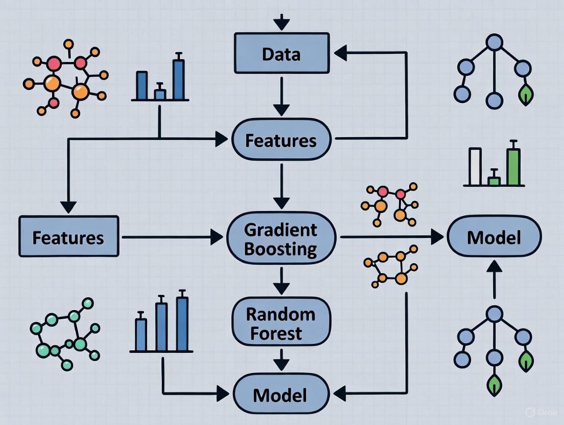
Workflow Visualization
Standard DBTL Cycle
Machine Learning-Enhanced LDBT Cycle
FAQs: Core Concepts and Problem Definition
Q1: What are "combinatorial explosions" in metabolic engineering, and why are they a critical bottleneck?
In metabolic engineering, combinatorial explosions refer to the exponential increase in the number of genetic variant combinations that need to be tested when simultaneously optimizing multiple pathway components. As the number of components (e.g., genes, promoters, RBS) to be optimized increases, the number of permutations grows exponentially, rendering full factorial searches experimentally infeasible. This creates a major bottleneck in the development of microbial cell factories for producing chemicals, fuels, and pharmaceuticals [10].
Q2: How does a "low-data regime" affect machine learning applications in metabolic engineering?
A low-data regime describes a scenario where the number of available experimental data points (e.g., strain performance measurements) is very small relative to the complexity of the system being modeled. This is a common challenge in metabolic engineering where building and testing strains is time-consuming and expensive. In these regimes, complex models like deep neural networks often overfit and fail to generalize, whereas certain ensemble methods like gradient boosting and random forests have been shown to be more robust and perform better [11].
Q3: What is the advantage of using ensemble ML models like Gradient Boosting over traditional methods for this problem?
Ensemble ML models combine multiple weaker models to create a single, more robust, and accurate predictor. This is particularly advantageous in low-data regimes with complex, non-linear relationships often found in biological systems. Gradient boosting iteratively builds models to correct the errors of previous ones, making it highly effective at capturing complex patterns from limited data. Random forests reduce overfitting by averaging predictions from multiple decorrelated decision trees. A recent study demonstrated that both gradient boosting and random forest models outperform other methods in the low-data regime, showing robustness to training set biases and experimental noise [11].
Q4: How does the DBTL cycle integrate with machine learning for combinatorial pathway optimization?
The Design-Build-Test-Learn (DBTL) cycle is an iterative framework for metabolic engineering. Machine learning powerfully integrates into the "Learn" phase. In this phase, data from the "Test" phase is used to train an ML model. This model then informs the next "Design" phase, predicting which genetic combinations might yield improved performance. Using ML to guide these cycles helps to strategically explore the vast combinatorial space, focusing experimental effort on the most promising candidates [11].
Troubleshooting Guides
Problem 1: Poor Model Performance and Overfitting in Initial DBTL Cycles
Symptoms: Your machine learning model performs well on training data but poorly when predicting new strain designs. Predictions are inaccurate and do not lead to improved strains in the next cycle.
Solutions:
- Action: Prioritize simpler models and strong regularization.
- Details: In initial cycles with very little data, start with simpler models like Random Forests or Gradient Boosting with strong regularization parameters. These models are less prone to overfitting than deep neural networks. For Gradient Boosting, reduce the model complexity by using a smaller
max_depthfor trees and a higherl2_regularizationparameter [12] [11].
- Details: In initial cycles with very little data, start with simpler models like Random Forests or Gradient Boosting with strong regularization parameters. These models are less prone to overfitting than deep neural networks. For Gradient Boosting, reduce the model complexity by using a smaller
- Action: Implement early stopping.
- Details: Use early stopping during model training to halt the process as soon as performance on a hold-out validation set stops improving. This prevents the model from over-optimizing to the noise in the small training dataset [12].
- Action: Leverage cross-validation.
- Details: Use techniques like k-fold cross-validation to get a more reliable estimate of your model's performance and for more robust hyperparameter tuning, even with limited data [13].
Problem 2: Navigating Combinatorial Explosion with Limited Experimental Budget
Symptoms: The number of potential genetic variant combinations is impossibly large, and you can only build and test a small number of strains per DBTL cycle.
Solutions:
- Action: Apply smart diversification strategies.
- Details: Do not diversify all pathway components at once. Use prior knowledge to identify the most rate-limiting steps (e.g., promoters for key genes, homologs for a specific enzyme) and focus combinatorial libraries on these. Strategies include varying coding sequences (gene homologs), expression levels (promoters, RBS), and gene dosage [10].
- Action: Use an algorithmic recommendation system.
- Details: Employ an algorithm that uses the trained ML model's predictions to recommend a shortlist of the most promising strains for the next DBTL cycle. Research indicates that when the total number of strains you can build is limited, it can be more effective to start with a larger initial DBTL cycle to provide the ML model with a better foundational dataset [11].
Problem 3: Model Failure in Subsequent DBTL Cycles
Symptoms: The model was effective in the first few cycles but is no longer generating improved designs, or performance has plateaued.
Solutions:
- Action: Retrain the model with accumulated data.
- Details: Avoid using a static model. The model should be retrained at the beginning of each DBTL cycle using all available data from all previous cycles. This allows the model to continuously learn and refine its understanding of the genotype-phenotype landscape [11].
- Action: Check for data distribution shifts.
- Details: As DBTL cycles progress, the new strains being tested may occupy a different region of the combinatorial space than the initial strains. Ensure your training data is representative of the space you are trying to explore. If not, actively design experiments to fill knowledge gaps.
The following table summarizes key quantitative findings from a foundational study that simulated DBTL cycles to evaluate machine learning methods for combinatorial pathway optimization [11].
Table 1: Comparative Performance of ML Methods in Simulated Metabolic Engineering DBTL Cycles
| Machine Learning Method | Performance in Low-Data Regime | Robustness to Training Set Bias | Robustness to Experimental Noise | Key Strengths |
|---|---|---|---|---|
| Gradient Boosting | Outperforms other tested methods | Robust | Robust | High accuracy, handles complex non-linear relationships |
| Random Forest | Outperforms other tested methods | Robust | Robust | Reduces overfitting, stable performance |
| Deep Neural Networks | Lower performance | Less Robust | Less Robust | Data-hungry; prone to overfitting with small data |
| Linear Models | Lower performance | N/A | N/A | Interpretable but often too simple for biological complexity |
Detailed Experimental Protocol: ML-Guided DBTL Cycle
This protocol outlines the steps for implementing a single iteration of a machine learning-guided DBTL cycle for combinatorial pathway optimization.
Objective: To use machine learning (Gradient Boosting/Random Forest) to select the best set of strain variants to build and test in the next cycle, with the goal of maximizing product titer/yield while minimizing experimental effort.
Materials and Reagents:
- Strain Library: A library of characterized genetic parts (e.g., promoter libraries, RBS libraries, gene homologs).
- Microbial Chassis: The host organism (e.g., E. coli, S. cerevisiae).
- DNA Assembly Reagents: Enzymes and kits for molecular cloning (e.g., Gibson assembly, Golden Gate assembly).
- Analytical Equipment: HPLC, GC-MS, or spectrophotometer for quantifying target product and growth metrics.
Procedure:
Learn: Model Training and Validation
- Input Data Preparation: Compile a dataset from all previous cycles. The dataset should consist of feature vectors (e.g., genetic part combinations, promoter strengths) and corresponding target variables (e.g., product titer, yield, growth rate).
- Model Training: Train a Gradient Boosting or Random Forest model on the compiled dataset. Use a train/validation split (e.g., 80/20) or k-fold cross-validation.
- Hyperparameter Tuning: Optimize key parameters using the validation set or cross-validation.
- Performance Assessment: Evaluate the final model on the hold-out test set or via cross-validation to ensure it has not overfit.
Design: In Silico Prediction and Recommendation
- In Silico Library Generation: Use the trained model to predict the performance of a large, in silico library of all possible genetic combinations within the defined design space.
- Strain Selection: Run a recommendation algorithm to select the top N (e.g., 50-100) most promising strain designs from the in silico library for experimental construction. The selection can be based on the highest predicted performance, or can also incorporate exploration of uncertain regions to improve the model.
Build: Library Construction
- Strain Engineering: Use high-throughput DNA assembly and genome engineering techniques (e.g., CRISPR-based methods, multiplex automated genome engineering) to construct the selected N strain variants in the microbial host [10].
Test: Phenotypic Characterization
- Cultivation and Assay: Grow the constructed strains in a controlled, high-throughput format (e.g., microtiter plates).
- Data Collection: Measure key performance indicators (KPIs) such as product titer, yield, and cellular growth for each strain variant.
- Data Curation: Organize the new experimental data (genotype and phenotype) for the next "Learn" phase.
The cycle then repeats from step 1, incorporating the new data.
Workflow and Pathway Diagrams
DBTL Cycle with ML Integration
Combinatorial Diversification Strategies
Research Reagent Solutions
Table 2: Key Research Reagents and Tools for Combinatorial Pathway Engineering
| Reagent / Tool | Function / Description | Application in Workflow |
|---|---|---|
| Promoter & RBS Libraries | Pre-characterized sets of genetic parts with varying strengths to fine-tune gene expression levels. | Design: Used to create diversity in expression levels for pathway genes to balance flux [10]. |
| Gene Homolog Libraries | A collection of alternative coding sequences from different species for the same enzymatic function. | Design: Provides diversity in enzyme kinetics and stability to overcome rate-limiting steps [10]. |
| CRISPR-Cas Systems | Tools for precise and multiplexed genome editing. | Build: Enables simultaneous modification of multiple genomic loci to construct complex variant strains [10]. |
| DNA Assembly Kits (e.g., Gibson, Golden Gate) | Enzyme mixes for seamlessly assembling multiple DNA fragments. | Build: Essential for high-throughput construction of pathway variants and genetic constructs [10]. |
| Genome-Scale Metabolic Models (GEMs) | Computational models of entire cellular metabolism. | Learn/Design: Provides a structured knowledge base and can be used to generate initial hypotheses and constrain ML models [15]. |
Frequently Asked Questions
Q1: My single decision tree model is overfitting, especially with my limited dataset. What is the simplest ensemble method to fix this?
A1: Bagging (Bootstrap Aggregating) is an excellent starting point. It reduces model variance and overfitting by training multiple decision trees on different random subsets of your training data (drawn with replacement) and then averaging their predictions [16] [17]. The Random Forest algorithm is an extension of bagging that further improves performance by also randomly selecting a subset of features at each split, creating more diverse and robust trees [16] [18].
Q2: I have a model where even small errors are costly. I want to sequentially improve my model's performance by focusing on hard-to-predict samples. Which method should I use?
A2: Boosting is designed for this exact scenario. Unlike bagging which runs models in parallel, boosting builds models sequentially, with each new model focusing on the errors made by the previous ones [17] [19]. Gradient Boosting, in particular, is a powerful technique that fits new models to the residual errors of the current ensemble, effectively minimizing the overall loss function in a gradient descent fashion [20] [21].
Q3: In a low-data regime, is it better to use Bagging or Boosting?
A3: Both can be adapted, but their approaches differ. Bagging uses bootstrap samples (random subsets with replacement) to create multiple training sets from a single limited dataset, allowing you to simulate a larger data environment [16] [22]. Boosting works sequentially to get the most out of every data point by concentrating on misclassified instances in each iteration [19]. In practice, the choice depends on your specific data and problem; empirical testing with cross-validation is often necessary to determine which performs better for your use case.
Q4: My ensemble model is becoming too complex and slow to train. How can I prevent overfitting and manage training time?
A4:
- For Gradient Boosting: Use early stopping. Monitor the model's performance on a validation set and halt training when performance stops improving [20]. Also, tune the learning rate; a smaller learning rate often requires more trees but can lead to better generalization [20].
- For Random Forest: While generally more resistant to overfitting, you can control complexity by tuning hyperparameters like
max_depth(maximum tree depth) andmin_samples_leaf(minimum samples required at a leaf node) [18]. Leverage Out-of-Bag (OOB) samples as an internal validation set to estimate performance without needing a separate dataset [16] [18].
Q5: How can I combine fundamentally different models (e.g., a decision tree and a logistic regression) for better performance?
A5: Use Stacking (Stacked Generalization). This advanced technique involves training multiple different (heterogeneous) base models in parallel. Then, their predictions are used as input features to train a final meta-model (e.g., a linear regression) that learns how to best combine the base models' predictions [17] [19]. A related technique called Blending uses a small holdout set instead of cross-validation for this last step [17].
The Scientist's Toolkit: Essential Algorithms & Libraries
The table below details key algorithms and libraries for implementing ensemble methods in a research environment.
| Name | Type | Primary Function | Key Consideration for Low-Data Regimes |
|---|---|---|---|
| Random Forest [16] [18] | Bagging | Creates an ensemble of decorrelated decision trees via bagging and feature randomness. | Bootstrap sampling efficiently utilizes limited data. OOB error provides a reliable validation estimate [16]. |
| Gradient Boosting (GBM) [20] [21] | Boosting | Sequentially builds an ensemble by fitting new models to the residual errors of the current ensemble. | Highly effective but requires careful tuning (learning rate, tree depth) and techniques like early stopping to prevent overfitting [20]. |
| AdaBoost [17] [19] | Boosting | An early boosting algorithm that re-weights misclassified data points for subsequent models. | Simpler than GBM, can be a good baseline. Focuses on hard examples, which can be beneficial with limited data. |
| Scikit-learn [17] | Library | Provides easy-to-use implementations for Random Forest, AdaBoost, and a basic Gradient Boosting classifier/regressor. | Ideal for prototyping and comparing different ensemble methods with a consistent API. |
| XGBoost [20] | Library | Optimized implementation of Gradient Boosting designed for speed and performance. | Often achieves state-of-the-art results. Excellent for fine-tuning and computational efficiency. |
| LightGBM [20] | Library | Another high-performance Gradient Boosting framework using novel techniques for faster training on large datasets. | Can be more efficient than XGBoost in some scenarios, useful when computational resources are a constraint. |
Experimental Protocols & Comparisons
Comparative Analysis of Bagging vs. Boosting
This table summarizes the core methodological differences between the two main ensemble paradigms, which is critical for selecting the right approach for an experiment.
| Aspect | Bagging (e.g., Random Forest) | Boosting (e.g., Gradient Boosting) |
|---|---|---|
| Core Objective | Reduce variance and overfitting [16] [22] | Reduce bias and improve accuracy [17] [19] |
| Data Sampling | Bootstrap samples (random with replacement); each model sees a different data subset [16] [17] | Whole dataset, but instances are re-weighted or errors are focused on sequentially [19] [22] |
| Model Training | Parallel and independent [19] | Sequential and dependent [19] |
| Base Model Type | Typically high-variance, complex models (e.g., deep decision trees) [16] | Typically high-bias, simple models (e.g., shallow decision trees/stumps) [22] |
| Aggregation | Averaging (regression) or Majority Voting (classification) [17] | Weighted averaging based on model performance [17] |
Visual Workflow: Bagging vs. Boosting
The diagram below illustrates the fundamental structural differences in the workflows for Bagging and Boosting algorithms.
Workflow comparison of parallel Bagging versus sequential Boosting.
Protocol: Implementing a Basic Gradient Boosting Regressor
This protocol outlines the key steps for implementing a Gradient Boosting model, which is particularly relevant for research in predictive modeling.
- Initialization: Start with a weak base learner (e.g., a decision tree with a single node). Make an initial prediction, which is often the average of the target values for regression [21].
- Loop for M iterations (one per new tree):
- Step A: Compute Residuals. For each instance in the training set, calculate the difference between the observed value and the current model's prediction. These are the negative gradients [20] [21].
- Step B: Fit a Weak Learner. Train a new weak learner (e.g., a decision tree) to predict these residuals. The tree is typically constrained by parameters like
max_depth(e.g., 3-8) [20]. - Step C: Update the Model. Add the new weak learner to the current ensemble. Its contribution is scaled by a
learning_rateparameter to prevent overfitting [20]. The update rule is:F_new(x) = F_old(x) + ν * h_m(x), whereνis the learning rate andh_m(x)is the new tree [21].
- Termination: The loop stops when a pre-set number of trees (
n_estimators) is reached, or when performance on a validation set stops improving (early stopping) [20].
Visual Workflow: Gradient Boosting Steps
The following diagram details the sequential, iterative process of the Gradient Boosting algorithm.
The iterative model correction process of Gradient Boosting.
Frequently Asked Questions (FAQs)
Q1: What exactly is meant by a "low-data regime" in machine learning for research? A: A "low-data regime" refers to situations where obtaining a large number of reliable, high-quality labeled data samples is challenging due to constraints such as time, cost, ethics, privacy, security, or technical limitations in data acquisition [23]. In such regimes, the number of training samples is so small that the ability of standard machine learning (ML) models to learn effectively sharply decreases, often resulting in poor predictive performance and a high risk of overfitting [23].
Q2: Between Gradient Boosting and Random Forest, which is more suitable for low-data scenarios? A: Random Forest is often recommended for initial low-data models because it is robust, fast to train, and less prone to overfitting due to its bagging approach, which builds multiple independent trees and averages their results [7]. Gradient Boosting, while often achieving higher accuracy, is more prone to overfitting with noisy or limited data and requires careful hyperparameter tuning, which can be difficult without sufficient data for validation [7]. For a very small number of labeled samples (e.g., few dozen), specialized multi-task learning approaches may be necessary [24].
Q3: What are the common pitfalls when applying Gradient Boosting to imbalanced datasets with low event rates? A: The primary pitfall is not the algorithm itself but using inappropriate evaluation metrics. With low event rates (e.g., 1%), metrics like Accuracy can be misleading [25]. It is crucial to use metrics like Area Under the Precision-Recall Curve (AUCPR) or Brier score, which provide a more accurate picture of model performance [25]. Furthermore, the predicted probabilities from Gradient Boosting models may need calibration to reliably capture tendencies in the data [25].
Q4: My dataset has multiple related properties, but each has very few measurements. How can I build a reliable model? A: Multi-task Learning (MTL) is designed for this scenario. It leverages correlations among related properties (tasks) to improve predictive performance for each individual task [24]. However, with imbalanced data, classical MTL can suffer from "negative transfer," where updates from one task harm another. Advanced training schemes like Adaptive Checkpointing with Specialization (ACS) can mitigate this by saving task-specific model checkpoints to protect against detrimental interference [24].
Q5: What practical steps can I take to improve model performance when my labeled data is severely limited? A: Several advanced ML strategies have been developed specifically for low-data challenges [23]:
- Transfer Learning: Initialize a model with knowledge from a related, data-rich domain and fine-tune it on your small dataset.
- Data Augmentation: Create new, synthetic training samples based on physical models or knowledge of the domain [23].
- Self-Supervised Learning (SSL): The model generates its own labels from the structure of unlabeled data, learning useful representations before fine-tuning on the limited labeled data [23].
- Semi-Supervised Learning: Leverage any available unlabeled data in addition to the small set of labeled data to improve learning [23].
Troubleshooting Guides
Issue 1: Model Performance is Poor on a Small, Imbalanced Dataset
Problem: Your Gradient Boosting or Random Forest model fails to produce meaningful outputs or shows poor predictive power on a dataset with a low event rate.
| Step | Action | Diagnostic Question | Solution / Next Step |
|---|---|---|---|
| 1 | Evaluate Metrics | Are you using accuracy? | Switch to metrics robust to imbalance: AUCPR, Brier Score, or F1-Score [25]. |
| 2 | Check Data Balance | What is the ratio of minority to majority class? | Employ stratified sampling or assign inverse prior weights during training [25]. |
| 3 | Validate Model Calibration | Are the predicted probabilities reliable? | Apply probability calibration techniques (e.g., Platt scaling, isotonic regression) to the model's output [25]. |
| 4 | Simplify the Model | Is the model overfitting? | For Random Forest, reduce tree depth. For Gradient Boosting, increase regularization, use a lower learning rate, or perform hyperparameter tuning [7]. |
Issue 2: Multi-Task Learning is Underperforming or Harming Individual Tasks
Problem: You are using MTL to jointly predict several molecular properties, but the overall performance is worse than training separate models.
| Step | Action | Diagnostic Question | Solution / Next Step |
|---|---|---|---|
| 1 | Identify Negative Transfer | Is performance on a specific task dropping during training? | Implement a training scheme like Adaptive Checkpointing (ACS) that saves task-specific model parameters to avoid detrimental updates [24]. |
| 2 | Analyze Task Relatedness | Are the tasks truly related? | Quantify task similarity. If tasks are unrelated, consider using separate models or a architecture with higher capacity to learn divergent tasks [24]. |
| 3 | Address Data Imbalance | Do the tasks have vastly different amounts of data? | Techniques like loss masking for missing labels can help, but advanced methods like ACS are specifically designed to handle severe task imbalance [24]. |
Quantitative Data on Low-Data Performance
The table below summarizes quantitative benchmarks for low-data regime performance from published research, providing a practical reference for expectations.
Table 1: Performance Benchmarks in Low-Data Regimes
| Dataset / Context | Model / Method | Data Scale | Key Performance Result | Reference |
|---|---|---|---|---|
| Molecular Property Prediction (e.g., ClinTox, SIDER) | Adaptive Checkpointing with Specialization (ACS) | As few as 29 labeled samples | Enabled accurate prediction of sustainable aviation fuel properties; outperformed single-task learning by 8.3% on average [24]. | [24] |
| General Small Data Challenges | Traditional ML (RF, SVM) vs. Deep Learning (CNN, ANN) | Very few training samples | DL models face severe overfitting; strategies like Transfer Learning, Data Augmentation, and Combining DL with traditional ML are essential [23]. | [23] |
| Imbalanced Dataset Classification | Gradient Boosting Machines | ~1.2% event rate in >4M samples | Model failed with default settings; required stratified sampling and inverse prior weights, highlighting sensitivity to imbalance [25]. | [25] |
Experimental Protocol: Implementing ACS for Multi-Task Learning
Objective: To train a robust multi-task graph neural network (GNN) on a dataset with severely imbalanced labels across tasks, mitigating negative transfer.
Materials:
- Dataset: A multi-task molecular property dataset (e.g., ClinTox, SIDER, or Tox21 from MoleculeNet).
- Software Framework: Python with deep learning libraries (e.g., PyTorch, Deep Graph Library).
- Computing Resources: GPU-enabled computing environment.
Methodology:
- Architecture Setup:
Training Loop:
- Train the entire model (shared backbone + all heads) on all tasks simultaneously.
- Monitor the validation loss for each individual task separately.
Adaptive Checkpointing:
- Throughout training, whenever the validation loss for a specific task reaches a new minimum, checkpoint (save) the current shared backbone parameters along with that task's specific head parameters [24].
- This ensures each task retains the best model state that worked for it, even if subsequent training updates are harmful.
Specialization:
- After training is complete, for each task, load its corresponding best-performing checkpoint to create a specialized model for deployment [24].
Workflow Visualization
Low-Data Modeling Strategy Selection
The Scientist's Toolkit: Research Reagent Solutions
Table 2: Essential Computational Tools for Low-Data Regime Research
| Tool / Technique | Function in Low-Data Research | Key Consideration |
|---|---|---|
| Random Forest | Provides a robust, fast baseline model. Less prone to overfitting, making it a safe first choice for exploration [7]. | Performance may plateau; less effective at capturing complex, sequential dependencies compared to boosting methods [7]. |
| Gradient Boosting | Offers high predictive power and flexibility. Can handle complex, non-linear relationships if tuned correctly [7]. | Highly sensitive to hyperparameters and noisy data. Requires more computational resources and expertise to avoid overfitting [7] [25]. |
| Multi-Task Learning (MTL) | Alleviates data bottlenecks by leveraging correlations among related tasks, improving data efficiency [24]. | Risk of "Negative Transfer" if tasks are not sufficiently related or data is severely imbalanced [24]. |
| Adaptive Checkpointing (ACS) | A training scheme that mitigates negative transfer in MTL, allowing reliable modeling with ultra-low data (e.g., <30 samples per task) [24]. | Increases training complexity and requires careful monitoring of validation loss for each task [24]. |
| Transfer Learning | Uses knowledge from a data-rich source task to improve learning on a low-data target task, effectively expanding the useful training set [23]. | Success depends on the relatedness between the source and target domains. |
| Self-Supervised Learning (SSL) | Learns useful data representations from unlabeled data, which can then be fine-tuned with limited labels, maximizing utility from available data [23]. | Requires defining a "pretext task" for the model to solve on unlabeled data. |
Frequently Asked Questions
FAQ: Machine Learning in Metabolic Engineering
Q1: Which machine learning methods are most effective for metabolic pathway optimization with limited experimental data?
A1: In low-data regimes commonly encountered in early-stage metabolic engineering, gradient boosting and random forest models have been demonstrated to outperform other machine learning methods. These approaches are particularly valuable because they show robustness to training set biases and experimental noise, which are common challenges with small datasets. Furthermore, when the number of strains you can build is limited, starting with a larger initial Design-Build-Test-Learn (DBTL) cycle is more favorable than distributing the same number of strains equally across all cycles [11].
Q2: What is a DBTL cycle and how does machine learning integrate with it?
A2: The Design-Build-Test-Learn (DBTL) cycle is an iterative framework for strain optimization in metabolic engineering. Its purpose is to progressively develop a production strain by incorporating learning from each previous cycle, thereby avoiding the "combinatorial explosion" that occurs when simultaneously optimizing many pathway genes. Machine learning integrates into this cycle by using data from the "Test" phase to "Learn" and propose improved genetic "Designs" for the next iteration, creating a data-driven feedback loop [11] [26].
Q3: How can I predict the activity of a novel compound for a specific biological target?
A3: This is achieved through Quantitative Structure-Activity Relationship (QSAR) modeling. QSAR models mathematically link a compound's molecular structure, represented by numerical descriptors, to its biological activity. You can train a model on a dataset of known compounds and then use it to predict the activity of new, unseen compounds. For critical tasks like predicting activity against a specific target (e.g., DHODH or TYMS in cancer research), support vector machines (SVM) with radial basis functions have shown high predictive performance (R² > 0.8 on unseen data) [27].
Q4: What are the common pitfalls when building a QSAR model and how can I avoid them?
A4: Common pitfalls include:
- Overfitting: Building a model that memorizes the training data but fails on new compounds. Solution: Use feature selection to reduce the number of descriptors and rigorously validate the model with a separate test set and cross-validation [28] [29].
- Poor Data Quality: Models are only as good as the data they are trained on. Solution: Carefully curate your dataset by removing duplicates, standardizing chemical structures, and handling missing values appropriately [28] [30].
- Ignoring the Applicability Domain: Using the model to predict compounds that are structurally very different from its training set. Solution: Define the chemical space of your training data and only apply the model to new compounds within that domain [28].
FAQ: QSAR Modeling
Q5: My QSAR model performs well on the training data but poorly on the test set. What is wrong?
A5: This is a classic sign of overfitting. Your model has likely learned the noise in the training data rather than the generalizable relationship between structure and activity. To address this:
- Simplify the model: Reduce the number of molecular descriptors using feature selection techniques.
- Use cross-validation: Tune your model's hyperparameters based on cross-validation performance within the training set, not on the test set.
- Gather more data: If possible, increase the size and diversity of your training dataset [28] [29].
Q6: What software tools are available for calculating molecular descriptors for QSAR?
A6: Several software packages can calculate a wide array of molecular descriptors. Common tools include:
- RDKit and Mordred (Open-source)
- PaDEL-Descriptor (Open-source)
- Dragon (Commercial)
- ChemAxon (Commercial) [28]
Troubleshooting Guides
Problem: Low Predictive Accuracy in a QSAR Model Built with a Small Dataset
This guide addresses the challenge of building a reliable QSAR model when you have a limited amount of bioactivity or property data.
| Step | Action | Rationale & Technical Details |
|---|---|---|
| 1 | Apply Data Augmentation | For deep learning models, represent each compound with multiple valid SMILES strings. The Maxsmi approach demonstrates that this augmentation improves model accuracy and allows the prediction's standard deviation across different SMILES to serve as an uncertainty measure [31]. |
| 2 | Select Robust Algorithms | Prioritize Gradient Boosting or Random Forest algorithms. These ensemble methods are known to perform well in low-data regimes and are less prone to overfitting compared to more complex models like deep neural networks on small datasets [11]. |
| 3 | Use Simple Descriptors | Calculate a manageable set of 200+ molecular descriptors (e.g., constitutional, topological) using tools like RDKit. Avoid generating thousands of complex descriptors that can easily lead to overfitting when data is scarce [29]. |
| 4 | Implement Rigorous Validation | Use k-fold cross-validation on your training data for model selection and keep a strict hold-out test set for final evaluation. This provides a more reliable estimate of how the model will perform on new, unseen compounds [28]. |
Problem: Inefficient DBTL Cycles for Combinatorial Pathway Optimization
This guide helps optimize the DBTL process when faced with a vast combinatorial space of possible genetic modifications.
| Symptom | Possible Cause | Solution |
|---|---|---|
| Slow progress between cycles; learning does not effectively inform next designs. | The learning phase is not systematically leveraging data to propose high-potential designs. | Integrate a machine learning recommendation algorithm. Use model predictions to guide the selection of which strains to build in the next cycle, focusing resources on the most promising parts of the design space [11]. |
| High experimental noise obscuring the signal from genetic changes. | The "Test" data is too variable, making it difficult for ML models to discern meaningful patterns. | Ensure experimental replicates and use ML methods like random forest which are demonstrated to be robust to a certain level of experimental noise [11]. |
| Limited number of strains can be built per cycle. | Resources are spread too thinly across many cycles. | Allocate a larger proportion of your total resources to the initial DBTL cycle. A larger initial dataset provides a stronger foundation for the ML model to learn from, which is more efficient than many small cycles [11] [32]. |
Experimental Protocols & Data
Protocol 1: Building a Basic QSAR Model using Random Forest
This protocol provides a step-by-step methodology for constructing a predictive QSAR model [29].
- Define Goal & Curate Data: Compile a dataset of chemical structures (as SMILES strings) and their associated biological activities (e.g., IC50, pIC50). Clean the data by standardizing structures and removing duplicates.
- Calculate Molecular Descriptors: Use a software tool like RDKit to compute numerical descriptors (e.g., molecular weight, logP, topological indices) for every compound in the dataset.
- Split Data: Divide the dataset into a training set (e.g., 80%) for model building and a test set (e.g., 20%) for final validation. The test set must be held out and not used in any model training.
- Train Model: Train a Random Forest model on the training set, using the molecular descriptors as features and the biological activity as the target variable.
- Validate Model: Use the trained model to predict the activity of the compounds in the test set. Calculate performance metrics (e.g., R², RMSE) by comparing predictions to the true values.
Workflow: QSAR Model Building
Protocol 2: Implementing an ML-Driven DBTL Cycle for Pathway Optimization
This protocol outlines how to integrate machine learning into iterative metabolic engineering cycles [11] [26].
- Design: Based on prior knowledge or ML recommendations, design a library of genetic variants (e.g., with different promoter/gene combinations).
- Build: Use molecular biology techniques to construct the designed strains.
- Test: Ferment the constructed strains and measure the output metrics (e.g., metabolite titer, yield, productivity).
- Learn: Use the collected "Build" and "Test" data to train a machine learning model (e.g., Gradient Boosting) to predict strain performance from genetic design.
- Recommend: Use the trained ML model to predict the performance of new, untested genetic designs and select the most promising ones for the next "Design" phase.
Workflow: ML-Driven DBTL Cycle
Table 1: Machine Learning Algorithm Performance in Low-Data Regime Metabolic Engineering [11]
| Algorithm | Performance in Low-Data Regime | Key Strengths |
|---|---|---|
| Gradient Boosting | Outperforms other methods | Robust to noise and training set bias. |
| Random Forest | Outperforms other methods | Robust to noise and training set bias. |
| Other Tested ML Methods | Lower performance | Less effective with limited data. |
Table 2: Key Research Reagent Solutions for Featured Experiments
| Reagent / Tool | Function / Application |
|---|---|
| gmctool (R application) | Identifies metabolic vulnerabilities in cancer cells by calculating genetic Minimal Cut Sets (gMCSs) using RNA-seq data [27]. |
| TCGAbiolinks (R library) | Retrieves and preprocesses transcriptomic data (e.g., RNA-seq) from The Cancer Genome Atlas (TCGA) for analysis [27]. |
| PaDEL-Descriptor, RDKit | Software tools to calculate molecular descriptors from chemical structures for QSAR modeling [28]. |
| OECD QSAR Toolbox | Software that supports chemical hazard assessment through read-across and categorization, incorporating metabolic simulators [33]. |
| Uni-QSAR (Auto-ML Tool) | An automated machine learning tool that combines multiple molecular representations (1D, 2D, 3D) for improved molecular property prediction [34]. |
Implementing Gradient Boosting and Random Forest in Your Research Pipeline
Gradient Boosting Machines (GBMs) represent a powerful machine learning ensemble technique that builds models sequentially, with each new model correcting the errors of its predecessors. In the context of drug development and research operating in low-data regimes (DBTL cycles - Design, Build, Test, Learn), GBMs offer particular advantages due to their ability to capture complex patterns from limited datasets. This technical support guide addresses the specific challenges researchers and scientists face when implementing GBMs in resource-constrained environments.
Core Concepts and Terminology
What is Gradient Boosting?
Gradient boosting is an ensemble learning method that builds models sequentially, where each new model in the sequence focuses on correcting the errors made by the previous models [35]. The algorithm combines multiple weak learners (typically decision trees) to create a strong predictive model [36]. This approach differs fundamentally from parallel ensemble methods like Random Forests, where trees are built independently [37].
Key Mechanism: Sequential Residual Modeling
The fundamental principle behind gradient boosting involves iteratively fitting new models to the residuals (errors) of the previous ensemble [38]. In regression tasks with squared error loss, this translates to directly modeling the differences between observed values and current predictions [39]. For other loss functions, the algorithm fits to pseudo-residuals, which represent the negative gradient of the loss function [21].
Frequently Asked Questions (FAQs)
How does gradient boosting differ from random forests?
The table below summarizes the key differences between these two popular ensemble methods:
| Feature | Gradient Boosting | Random Forest |
|---|---|---|
| Model Building | Sequential, trees built one after another [37] | Parallel, trees built independently [37] |
| Bias-Variance | Lower bias, higher variance thus more prone to overfitting [37] | Lower variance, less prone to overfitting [37] |
| Training Approach | Each new tree corrects errors of previous ones [38] | Each tree built on random data and feature subsets [37] |
| Training Time | Slower due to sequential nature [37] | Faster due to parallel training [37] |
| Robustness to Noise | More sensitive to outliers and noise [37] | Less sensitive to outliers and noise [37] |
| Hyperparameter Sensitivity | High sensitivity requires careful tuning [37] | Less sensitive, more robust to suboptimal settings [37] |
When should I choose gradient boosting over random forests in low-data regimes?
For DBTL research with limited data, consider gradient boosting when:
- High predictive accuracy is crucial and you have relatively clean data [37]
- You need to capture complex nonlinear relationships in small to medium datasets [14]
- You have computational resources for extensive hyperparameter tuning [37]
- Interpretability is secondary to pure predictive performance [37]
What are the most critical hyperparameters to tune in gradient boosting?
The most impactful hyperparameters include:
- Learning rate: Controls contribution of each tree (typical range: 0.001-0.3) [39]
- Number of trees: Too few underfit, too many overfit [35]
- Tree depth: Controls model complexity (1-6 splits common for weak learners) [39]
- Minimum samples split: Prevents overfitting by limiting node splits [35]
Troubleshooting Guides
Problem: Model Overfitting in Small Datasets
Symptoms:
- Excellent training performance but poor validation results
- Large gap between training and validation metrics
- Unrealistic predictions on new data
Solutions:
- Increase regularization: Reduce tree depth, increase minimum samples per leaf
- Lower learning rate: Use values between 0.01-0.1 with more trees [40]
- Apply shrinkage: Scale the contribution of each tree [40]
- Use early stopping: Halt training when validation performance plateaus [35]
- Implement stochastic boosting: Use random subsamples of data for each tree [39]
Experimental Protocol:
Symptoms:
- Experiment iteration cycles become impractically long
- Hyperparameter tuning consumes excessive resources
- Model development delays DBTL cycles
Solutions:
- Use shallower trees: Limit depth to 2-4 for faster computation [39]
- Reduce feature space: Apply feature selection prior to modeling
- Implement early stopping: Avoid unnecessary iterations [35]
- Leverage GPU acceleration: Use implementations like XGBoost with GPU support
- Start with smaller subsets: Prototype with data samples before full training
Problem: Handling Noisy Data in Experimental Measurements
Symptoms:
- Model performance fluctuates significantly with small data changes
- High sensitivity to measurement outliers
- Inconsistent feature importance rankings
Solutions:
- Use robust loss functions: For regression, consider Huber loss instead of MSE [41]
- Increase bagging fraction: Use smaller subsamples to reduce outlier impact
- Apply feature scaling: Normalize or standardize input features
- Implement cross-validation: Use robust performance estimation strategies
- Remove extreme outliers: Preprocess data to remove measurement errors
Workflow Visualization
Gradient Boosting Sequential Training Process
Bias-Variance Tradeoff in Sequential Learning
The Researcher's Toolkit: Essential Components
Key Hyperparameters and Their Functions
| Component | Function | Impact on Low-Data Regimes |
|---|---|---|
| Learning Rate | Controls contribution of each tree to the ensemble [40] | Critical for preventing overfitting; lower values (0.01-0.1) preferred with limited data |
| Tree Depth | Determines complexity of individual weak learners [39] | Shallower trees (2-4 levels) reduce variance in small datasets |
| Number of Trees | Total iterations in the sequential process [35] | Requires careful tuning; too many trees overfit small datasets |
| Subsample Ratio | Fraction of data used for each tree (stochastic boosting) [39] | Introduces diversity and reduces overfitting in limited data |
| Minimum Samples Split | Smallest number of observations required to split a node [35] | Higher values prevent modeling noise in small datasets |
Experimental Design Considerations for DBTL Research
When implementing gradient boosting in low-data drug development contexts:
- Prioritize Cross-Validation: Use leave-one-out or repeated k-fold CV for reliable performance estimation [23]
- Focus on Regularization: Emphasize hyperparameters that control model complexity
- Implement Early Stopping: Automate stopping criteria to prevent overfitting [35]
- Leverage Domain Knowledge: Incorporate biological constraints into feature engineering
- Plan Iterative Refinement: Design experiments to sequentially improve data quality
Advanced Techniques for Low-Data Environments
Transfer Learning Applications
In DBTL frameworks where initial data is scarce, transfer learning can help leverage related domains or previous experiments to bootstrap models [23]. Pre-training on larger public datasets followed by fine-tuning on specific experimental data can improve performance in data-limited scenarios.
Hybrid Modeling Approaches
Combining gradient boosting with traditional machine learning models or physical models can enhance performance when data is limited [23]. These hybrid approaches leverage both data-driven patterns and domain knowledge to compensate for small sample sizes.
Performance Optimization Checklist
- Implement early stopping to prevent overfitting
- Use learning rate values between 0.01-0.1 for small datasets
- Limit tree depth to 2-4 for weak learners
- Apply stochastic boosting with subsampling
- Use robust cross-validation strategies
- Regularize using minimum samples per split/leaf
- Monitor training vs validation performance gaps
- Consider robust loss functions for noisy experimental data
By understanding these core principles, troubleshooting common issues, and implementing the recommended strategies, researchers can effectively leverage gradient boosting in DBTL cycles and low-data regime research to advance drug development initiatives.
Frequently Asked Questions (FAQs)
Q1: My Random Forest model performs nearly perfectly on training data but poorly on test data. Am I overfitting, and how can I prevent this?
Yes, this indicates overfitting. To prevent it:
- Tune Hyperparameters: Optimize parameters that control tree growth, such as:
mtry: The number of features to consider at each split.nodesizeormin_samples_leaf: The minimum number of samples required to be at a leaf node.max_depth: The maximum depth of the tree [42].
- Use Correct Training Performance Metric: For the training data, always use the Out-of-Bag (OOB) error, an unbiased estimate calculated from samples not used to build a given tree. Do not use
predict(model, newdata=train), which creates artificially high scores [42]. - Employ Cross-Validation: Use k-fold cross-validation to robustly evaluate model performance and guide hyperparameter tuning [42].
Q2: Why are my Random Forest regression predictions never outside the range of the target values seen in the training data?
This is a fundamental characteristic of the algorithm. A Random Forest for regression averages the predictions of its individual decision trees [43] [44]. Each tree's prediction is the mean of the samples in a leaf node [45]. Therefore, the final averaged prediction cannot exceed the maximum or minimum values present in the training set. Random Forests are poor at extrapolating outside the training data range [45]. For tasks requiring trend extrapolation, consider linear models, Support Vector Regression (SVR), or neural networks [45].
Q3: In a low-data regime for drug-target interaction (DTI) prediction, how can I make the most of Random Forest?
- Leverage Bootstrap Aggregation: The inherent bagging in Random Forest is beneficial for low-data scenarios. Each tree is trained on a different bootstrap sample of the limited data, effectively creating diversity and making the ensemble more robust [43] [46].
- Prioritize Feature Selection: Use feature selection techniques (e.g., based on XGBoost importance or domain knowledge) to reduce the feature space before training the Random Forest. This prevents overfitting and improves model focus on the most relevant molecular descriptors [47].
- Innovative Feature Engineering: Create powerful, informative features. For example, one study used 3D molecular fingerprints and transformed molecular similarity matrices into probability distributions using Kullback-Leibler divergence (KLD) as features for the Random Forest, achieving high accuracy in DTI prediction even with a limited number of targets [48].
Troubleshooting Guide
| Problem | Symptom | Likely Cause | Solution |
|---|---|---|---|
| Overfitting | High accuracy/AUC on training set (>99%), but significantly lower performance on test/hold-out set [42]. | Trees grown too deep without sufficient regularization; model learns noise in training data. | Increase min_samples_leaf or nodesize. Increase max_depth restriction. Tune mtry via cross-validation [42]. |
| Poor Extrapolation | Regression predictions for new data are consistently constrained within the min/max range of the training target values [45]. | Algorithmic limitation; predictions are averages of training data outcomes. | Use an alternative model (Linear Regression, SVR) or a hybrid/stacked model that combines Random Forest with a linear algorithm [45]. |
| Low Predictive Accuracy | Model performance is poor on both OOB/test samples and new validation data. | Uninformative features, noisy data, or suboptimal hyperparameters. | Perform feature selection and engineering. Optimize all key hyperparameters (mtry, nodesize, n_estimators) using grid/random search with cross-validation. |
| Long Training Times | Model takes excessively long to train, especially on larger datasets. | Large number of trees (n_estimators), large dataset, or too many features considered at splits. |
Start with a smaller subset for prototyping. Use a computing environment with parallel processing, as Random Forest training can be parallelized [44]. |
Experimental Protocol: Predicting Drug-Target Interactions (DTI) in a Low-Data Regime
This protocol outlines a methodology for building a Random Forest model to predict interactions between drug compounds and biological targets, which is particularly relevant for drug repurposing and understanding polypharmacology in a low-data context [48].
Workflow Diagram
Key Steps
Data Curation:
Molecular Featurization:
Advanced Feature Engineering (KLD Features):
- Q-Q Matrix: For each target protein, compute the pairwise 3D similarity of all its known ligands. This matrix characterizes the target's "uniqueness" [48].
- Q-L Vector: For a query compound and a target, compute the pairwise 3D similarities between the query and all the target's known ligands [48].
- Use Kernel Density Estimation (KDE) to transform the similarity scores of both the Q-Q matrix and Q-L vectors into probability density functions.
- Calculate the Kullback-Leibler divergence (KLD) between the Q-L vector's distribution and the Q-Q matrix's distribution. The KLD serves as a "quasi-distance" and becomes the novel, powerful feature vector for the Random Forest classifier [48].
Model Training and Validation:
Performance Data
Comparative Algorithm Performance in Drug Discovery
| Algorithm | Application Context | Key Performance Metric | Result | Reference |
|---|---|---|---|---|
| Random Forest | Anti-breast cancer drug candidate bioactivity prediction | Prediction Accuracy | 0.745 | [47] |
| XGBoost | Anti-breast cancer drug candidate bioactivity prediction | Prediction Accuracy | Comparable to RF | [47] |
| Gradient Boosting | Anti-breast cancer drug candidate bioactivity prediction | Prediction Accuracy | Comparable to RF | [47] |
| Support Vector Machine (SVM) | Anti-breast cancer drug candidate bioactivity prediction | Prediction Accuracy | Worst among tested | [47] |
| Random Forest (with KLD) | Drug-Target Interaction prediction for 17 targets | Mean Accuracy / OOB Score / ROC AUC | 0.882 / 0.876 / 0.990 | [48] |
The Scientist's Toolkit: Research Reagent Solutions
| Item | Function in the Experimental Protocol |
|---|---|
| ChEMBL Database | A public repository of bioactive molecules with drug-like properties, providing curated bioactivity data (e.g., IC50) for training the model [48]. |
| E3FP Fingerprint | A 3D molecular fingerprint that captures the radial distribution of atomic features around each atom, providing a comprehensive representation of a molecule's 3D structure for similarity calculations [48]. |
| Kullback-Leibler Divergence (KLD) | A statistical measure of how one probability distribution diverges from a second. It is used as a feature engineering tool to quantify the relationship between a query molecule and a target's ligand set [48]. |
| Out-of-Bag (OOB) Score | An unbiased internal validation metric for Random Forests. It estimates the model's prediction error using data points not included in the bootstrap sample for a given tree, reducing the need for a separate validation set [43]. |
Frequently Asked Questions (FAQs)
Algorithm Selection & Performance
Q: When should I choose Gradient Boosting over Random Forest in a low-data metabolic engineering context?
A: The choice depends on your data characteristics and priority. For small datasets composed mainly of categorical variables, Random Forest (bagging) often provides more stable and accurate predictions [49]. However, Gradient Boosting (boosting) can achieve excellent predictive performance for certain specific prediction tasks, despite being generally less stable on small data [49]. Empirical studies across 165 datasets confirm that both are top-performing ensemble methods, but neither is a universal winner [50].
Q: Why does my ML model perform poorly even after tuning, and how can I improve it?
A: Poor performance can stem from the fundamental "no free lunch" theorem in ML. Key improvement strategies include:
- Systematic Algorithm Spot-Checking: Test a suite of algorithms, as performance is problem-dependent [50].
- Comprehensive Hyperparameter Tuning: This can improve accuracy by 3-50%, depending on the algorithm and dataset [50].
- Feature Engineering: Model performance is significantly affected by the characteristics of the features used for development [49].
Implementation & Technical Issues
Q: What are the best practices for validating ML models on limited experimental data?
A: For small datasets, use Leave-One-Out Cross-Validation (LOOCV) [49]. LOOCV uses all samples for both training and testing, providing a robust performance estimate when data is scarce. Avoid simple train-test splits, which can be unreliable with limited samples.
Q: How can I integrate biosensor data effectively into my DBTL cycle for dynamic control?
A: Effectively integrate biosensors by characterizing their key performance parameters [51]:
- Dynamic Range and Operating Range: Ensure the biosensor covers the relevant metabolite concentrations.
- Response Time: Slow responses hinder real-time controllability.
- Signal-to-Noise Ratio: High noise obscures subtle metabolic differences. For dynamic regulation, consider hybrid approaches combining slower, stable systems with faster-acting components like riboswitches to improve overall performance [51].
Data Handling & Visualization
Q: How should I visualize high-dimensional ML results for metabolic engineering applications?
A: Follow these core principles for effective visualization [52]:
- Prioritize Clarity and Accuracy: Ensure visuals are easy to interpret and build trust.
- Provide Context: Use titles and annotations to explain the "so what".
- Know Your Audience: Tailor depth and presentation to researchers or decision-makers. Choose the chart type based on the story you need to tell. For model performance comparison, use bar charts. For tracking optimization across DBTL cycles, use line charts [52].
Q: My data is highly skewed. Will this negatively impact Random Forest or Gradient Boosting models?
A: Both Random Forest and Gradient Boosting can handle skewed data reasonably well compared to models like linear regression [53]. Their ensemble nature and built-in feature importance analysis provide robustness and interpretability with non-normally distributed data.
Troubleshooting Guides
Poor ML Model Accuracy
| Step | Action | Diagnostic Check |
|---|---|---|
| 1 | Verify Data Quality & Preprocessing | Check for outliers, perform normalization, and ensure proper handling of categorical variables [49]. |
| 2 | Spot-Check Multiple Algorithms | Test at least 5 different algorithms: Gradient Boosting, Random Forest, Support Vector Machines, Extra Trees, and Logistic Regression [50]. |
| 3 | Perform Hyperparameter Tuning | Use grid search or similar methods; tuning can yield 3-50% accuracy gains [50]. |
| 4 | Evaluate with Proper Validation | Use LOOCV for small datasets to ensure reliable performance estimates [49]. |
| 5 | Analyze Feature Importance | Use built-in functions from tree-based models to identify and focus on the most impactful features [49] [53]. |
Inconsistent Results Across DBTL Cycles
| Symptom | Possible Cause | Solution |
|---|---|---|
| High variance in model performance between cycles | Lack of standardized experimental protocols and data collection. | Implement Standard Operating Procedures (SOPs) for all experimental steps and data recording. |
| Model fails to generalize to new cycles | Overfitting to noise or specific conditions of initial cycles. | Increase dataset size via data augmentation, apply stronger regularization in ML models, and use ensemble methods. |
| Inability to compare results across cycles | Missing metadata and inconsistent context for data points. | Create a standardized metadata template capturing all relevant experimental conditions for each data point. |
Biosensor Integration Challenges
| Problem | Root Cause | Resolution |
|---|---|---|
| Slow or delayed response in dynamic control | Inherently slow biosensor response kinetics. | Implement hybrid approaches (e.g., combine with fast-acting riboswitches) or engineer biosensors for improved response time [51]. |
| High signal noise obscures metabolic differences | Non-optimal biosensor design or external interference. | Characterize signal-to-noise ratio, use filtering techniques, and employ biosensors with higher specificity [51]. |
| Limited detection window for metabolite concentrations | Biosensor dynamic/operating range mismatched with metabolite levels. | Re-select or engineer biosensors with an operating range that covers the required metabolite concentration window [51]. |
Experimental Protocols & Data
Standardized Protocol for Consistent ML Comparison
This protocol ensures fair and reproducible comparison of ML algorithms across simulated DBTL cycles in low-data regimes.
1. Data Preprocessing and Standardization
- Collect and preprocess data, eliminating outliers [49].
- Normalize or standardize features to ensure consistent scaling across variables [49].
- For categorical variables, use appropriate encoding techniques.
2. Model Training with Hyperparameter Tuning
- Select a diverse set of ML algorithms for initial spot-checking [50].
- For each algorithm, perform hyperparameter tuning using a defined grid of values [50].
- Use a consistent resampling method (e.g., 5-fold CV) during tuning for comparability [53].
3. Model Validation and Evaluation
- Evaluate final model performance using Leave-One-Out Cross-Validation (LOOCV) to maximize data usage in small-sample settings [49].
- Calculate a standard set of performance metrics: R² (coefficient of determination), RMSE (Root Mean Square Error), MAE (Mean Absolute Error), and Pearson's R [49].
- Rank algorithm performance on each dataset to identify the most suitable one [50].
ML Algorithm Performance in Low-Data Regimes
Table: Comparative performance of ensemble algorithms on small datasets, relevant to metabolic engineering applications.
| Algorithm | Ensemble Type | Key Strengths | Performance on Small Categorical Data | Considerations |
|---|---|---|---|---|
| Random Forest (RF) | Bagging | High stability, robust to outliers, handles imbalanced classes [49]. | Predictions are more stable and accurate [49]. | Less prone to overfitting; lower computational time [53]. |
| Gradient Boosting (GBM) | Boosting | Effectively reduces bias and variance, high predictive power when tuned [49]. | Can demonstrate excellent performance for specific tasks [49]. | Can be more sensitive to hyperparameters and noisy data [49]. |
Table: Results from a large-scale study comparing 13 algorithms across 165 datasets [50].
| Algorithm | Average Rank (Lower is Better) | Significance Group | Recommended for Initial Spot-Checking? |
|---|---|---|---|
| Gradient Boosting | 1 (Best) | Top Performer | Yes [50] |
| Random Forest | 2 | Top Performer | Yes [50] |
| Support Vector Machines | 3 | High Performer | Yes [50] |
| Extra Trees | 4 | High Performer | Yes [50] |
| Logistic Regression | 5 | High Performer | Yes [50] |
� Workflow & Pathway Visualizations
DBTL Cycle with Integrated ML Analysis
Bagging vs. Boosting Workflow
Research Reagent Solutions
Table: Key biosensor types for dynamic monitoring and control in metabolic engineering DBTL cycles [51].
| Reagent / Tool | Type | Primary Function in Metabolic Engineering |
|---|---|---|
| Transcription Factor (TF)-based Biosensors | Protein-based Sensor | Links metabolite concentration to measurable outputs (e.g., fluorescence) for high-throughput screening of strain libraries [51]. |
| Riboswitches | RNA-based Sensor | Provides dynamic, modular control of gene expression via ligand-induced conformational changes, enabling real-time regulation of metabolic fluxes [51]. |
| Two-Component Systems (TCSs) | Protein-based Sensor | Enables detection of extracellular/intracellular signals (ions, pH, small molecules) and signal transduction for environmental monitoring [51]. |
| Toehold Switches | RNA-based Sensor | Provides programmable, logic-gated control of metabolic pathways via RNA-RNA interaction, increasing production efficiency [51]. |
Troubleshooting Guides and FAQs
FAQ 1: Which gradient boosting implementation should I choose for my QSAR project?
The choice depends on your specific priorities regarding predictive performance, training speed, and dataset size [54].
- For the best predictive performance:
XGBoostis generally recommended, as it consistently achieved the best predictive performance in a large-scale benchmark study [54] [55]. - For the fastest training on large datasets:
LightGBMis the optimal choice, as it requires the least training time, making it ideal for high-throughput screening (HTS) data [54]. - For small datasets or to reduce overfitting risk:
CatBoostand its ordered boosting approach can be more robust, especially in low-data regimes [54].
FAQ 2: How can I prevent my model from overfitting, especially with a small dataset?
Overfitting is a common challenge, but several strategies can mitigate it [54] [56] [57].
- Apply Regularization: Utilize the built-in L1 (Lasso) and L2 (Ridge) regularization in algorithms like
XGBoostto penalize complex models [54] [56]. - Constrain the Trees: Limit the depth of the decision trees (
max_depth) and the number of leaves. Simpler, "weaker" trees are less prone to overfitting [56]. - Use Shrinkage: Incorporate a learning rate (shrinkage) to slow down the learning process, making the model more robust [56].
- Employ Stochastic Gradient Boosting: Train each tree on a random subset of the data (rows) and/or features (columns) to reduce the correlation between trees and improve generalization [56].
- Tune Hyperparameters Extensively: The relevance of each hyperparameter varies across datasets. Optimizing as many hyperparameters as possible is crucial for maximizing performance and avoiding overfitting [54].
FAQ 3: My dataset has many highly correlated molecular descriptors. Is this a problem?
Gradient Boosting models are inherently robust to descriptor intercorrelation (multi-collinearity) due to their decision-tree-based architecture, which naturally prioritizes informative splits and down-weights redundant descriptors [57]. This makes them well-suited for high-dimensional descriptor sets. However, if overfitting is still evident, you can:
- Use Recursive Feature Elimination (RFE): A supervised method that iteratively removes the least important descriptors based on model performance [57].
- Remove low-variance and highly correlated descriptors as a pre-processing step, though this may sometimes discard meaningful features [57].
FAQ 4: Can I trust the feature importance rankings from my model?
While gradient boosting models provide feature importance scores, they should be interpreted with caution. Different implementations (XGBoost, LightGBM, CatBoost) can surprisingly rank molecular features differently due to differences in their regularization techniques and decision tree structures [54]. Therefore, expert knowledge must always be employed when evaluating these data-driven explanations of bioactivity. The rankings are a useful guide, but not an absolute truth [54].
FAQ 5: How well does gradient boosting perform in a low-data regime?
Evidence suggests that gradient boosting can be effective even with limited data. One study on demolition waste prediction, which used a small dataset of 690 samples, found that while Random Forest (a bagging algorithm) provided more stable predictions, Gradient Boosting Machine (GBM) models demonstrated excellent predictive performance for some specific predictive tasks [58]. Furthermore, in the context of metabolic engineering, gradient boosting and random forest were shown to outperform other methods in the low-data regime for combinatorial pathway optimization [59].
Experimental Protocols & Data Presentation
Large-Scale Benchmarking Protocol for GBM Implementations
The following protocol is derived from a comprehensive study that trained 157,590 models on 16 datasets covering 94 endpoints and 1.4 million compounds [54].
1. Dataset Curation
- Compile datasets from reliable sources, ensuring they cover a diverse chemical space relevant to your problem [28].
- Standardize chemical structures (e.g., remove salts, normalize tautomers) [28].
- Handle missing values by either removing compounds or imputing values (e.g., with the column median) [60].
2. Molecular Descriptor Calculation
- Calculate a diverse set of 2D molecular descriptors using software like
RDKitorMordred[54] [60]. These can include constitutional, topological, and physicochemical descriptors [28].
3. Data Preprocessing
- Scale molecular descriptors to have zero mean and unit variance [28].
- Split the dataset into training and test sets. The external test set must be reserved exclusively for final model assessment [28].
4. Model Training and Hyperparameter Optimization
- For each GBM implementation (
XGBoost,LightGBM,CatBoost), perform hyperparameter tuning. The study found it crucial to optimize as many hyperparameters as possible [54]. - Key hyperparameters to tune include:
n_estimators: The number of boosting stages.max_depth: The maximum depth of the individual trees.learning_rate: The shrinking factor of the contribution of each tree.- Regularization parameters (e.g.,
reg_alphafor L1,reg_lambdafor L2 inXGBoost).
5. Model Validation
- Use k-fold cross-validation (e.g., 5-fold) on the training set to tune hyperparameters and prevent overfitting [28].
- Use the held-out external test set to provide a realistic estimate of the model's performance on unseen data [28].
6. Performance Evaluation
- For classification: Use metrics like Accuracy, Precision, Recall, and F1-score [60].
- For regression: Use metrics like R², Root Mean Squared Error (RMSE), and Mean Absolute Error (MAE) [61].
Performance Comparison of GBM Implementations and Other Algorithms
The tables below summarize quantitative findings from various studies, providing a clear comparison for model selection.
Table 1: Comparison of GBM implementations for general QSAR modeling based on a large-scale benchmark [54].
| Implementation | Key Strengths | Key Weaknesses/Trade-offs |
|---|---|---|
| XGBoost | Best overall predictive performance; strong regularization. | Slower training time compared to LightGBM. |
| LightGBM | Fastest training time, especially on large datasets. | Depth-first tree growth may overfit on small datasets. |
| CatBoost | Robust on small datasets; handles categorical features. | Target leakage prevention less relevant for standard molecular descriptors. |
Table 2: Algorithm performance in predicting Lung Surfactant Inhibition (a binary classification QSAR task) [60].
| Algorithm | Accuracy | F1-Score |
|---|---|---|
| Multilayer Perceptron (MLP) | 96% | 0.97 |
| Gradient-Boosted Trees (GBT) | Reported as lower than MLP | Reported as lower than MLP |
| Support Vector Machines (SVM) | High (but lower than MLP) | High (but lower than MLP) |
| Logistic Regression (LR) | High (but lower than MLP) | High (but lower than MLP) |
| Random Forest (RF) | Lower than MLP | Lower than MLP |
Table 3: Algorithm performance in a low-data regime (690 samples) for a regression task [58].
| Algorithm | Overall Finding | Contextual Performance |
|---|---|---|
| Random Forest (RF) | Predictions were more stable and accurate. | N/A |
| Gradient Boosting (GBM) | Less stable than RF overall. | Demonstrated excellent predictive performance for some specific waste types. |
Workflow and Relationship Visualizations
Gradient Boosting for QSAR in the DBTL Cycle
The following diagram illustrates how Gradient Boosting integrates into a Design-Build-Test-Learn (DBTL) cycle, which is central to low-data regime research in fields like metabolic engineering and drug discovery [59].
Core Gradient Boosting Algorithm Workflow
This diagram outlines the fundamental iterative process of the Gradient Boosting algorithm, showing how multiple weak learners (trees) are combined to create a strong predictive model [56].
The Scientist's Toolkit: Research Reagent Solutions
Table 4: Essential software and libraries for implementing Gradient Boosting in QSAR modeling.
| Tool Name | Type | Primary Function in QSAR |
|---|---|---|
| RDKit / Mordred | Cheminformatics Library | Calculates a large set of 2D and 3D molecular descriptors from chemical structures [60] [57]. |
| XGBoost | Machine Learning Library | A high-performance implementation of gradient boosting with strong regularization [54] [60]. |
| LightGBM | Machine Learning Library | A gradient boosting framework designed for efficiency and distributed training on large datasets [54]. |
| CatBoost | Machine Learning Library | A gradient boosting implementation specialized in handling categorical features and reducing overfitting [54]. |
| Scikit-learn | Machine Learning Library | Provides utilities for data preprocessing (e.g., scaling, imputation), model validation (e.g., cross-validation), and baseline models [60]. |
| Flare | Commercial Platform (Cresset) | An integrated software platform for structure-based design that includes built-in tools for creating Gradient Boosting QSAR models [57]. |
| PaDEL-Descriptor | Cheminformatics Software | An alternative software for calculating molecular descriptors [28]. |
Frequently Asked Questions
Q1: I am in the early stages of a DBTL cycle with very limited training data. Which algorithm is more suitable?
For the initial DBTL cycles where data is scarce, Random Forest is often the more stable and robust choice [49]. Its bagging technique, which builds trees independently on random subsets of the data, reduces variance and the risk of overfitting on small datasets [7] [37]. Evidence from metabolic engineering research confirms that both Random Forest and Gradient Boosting perform well in low-data regimes, but Random Forest predictions tend to be more stable [62].
Q2: My dataset has many categorical features with high cardinality. How do these algorithms handle this, and what pitfalls should I avoid?
This is a critical consideration. Standard Gradient Boosting implementations that use CART trees can be biased towards categorical variables with large cardinalities [63]. This bias can skew feature importance measures, leading to misinterpretations. If using Gradient Boosting with such data, seek out modern implementations like LightGBM, which natively support categorical features, or consider advanced frameworks like Cross-Validated Boosting (CVB) that mitigate this bias [63]. Random Forest is generally less prone to this issue.
Q3: I need the highest predictive accuracy possible and have time for tuning. Which algorithm should I invest in?
If predictive accuracy is the paramount goal and you have the computational resources and time for careful hyperparameter tuning, Gradient Boosting is likely to yield the highest performance [7] [37]. Its sequential error-correction mechanism allows it to capture complex patterns in the data. However, this comes at the cost of longer training times and a higher risk of overfitting, especially if your data is noisy [7] [64].
Q4: For a project in drug discovery, where interpretability of the model is important, which ensemble method is preferable?
Random Forest is generally more interpretable than Gradient Boosting [37]. It provides straightforward feature importance measures based on the average decrease in impurity across all trees, allowing researchers to understand which features (e.g., molecular descriptors) contribute most to predictions [37]. While Gradient Boosting models can also provide feature importance, it is often less intuitive due to the sequential, dependent nature of the trees [37].
Algorithm Comparison at a Glance
The table below summarizes the core characteristics of Gradient Boosting and Random Forest to guide your initial selection.
| Feature | Gradient Boosting | Random Forest |
|---|---|---|
| Core Principle | Builds trees sequentially to correct errors of previous trees [7] [37] | Builds trees independently and combines their outputs [7] [37] |
| Primary Strength | High predictive accuracy; handles complex relationships well [7] [37] | Robustness; resistance to overfitting; handles noisy data well [7] [64] [37] |
| Best for Data Size | Small to medium-sized, cleaner datasets [37] | Large datasets; highly scalable [7] [37] |
| Computational Cost | Higher training time (sequential) [7] [37] | Lower training time (parallelizable); faster predictions [7] [37] |
| Overfitting Risk | Higher, especially without regularization and on noisy data [7] [37] | Lower, due to averaging and feature randomness [7] [65] [37] |
| Hyperparameter Sensitivity | High (e.g., learning rate, tree depth) [7] [37] | Lower; more robust to suboptimal settings [37] |
| Interpretability | Lower; feature importance can be less straightforward [37] | Higher; provides clear feature importance measures [64] [37] |
Experimental Protocol for Algorithm Evaluation in a DBTL Context
This protocol is designed for a rigorous, unbiased comparison of the two algorithms within a resource-constrained research environment, such as early-stage drug discovery.
1. Hypothesis and Objective Definition
- Primary Objective: To determine which algorithm, Gradient Boosting or Random Forest, provides superior and more reliable predictive performance for a specific task (e.g., predicting drug sensitivity or metabolic yield) in the current low-data regime of our DBTL cycle.
- Success Metrics: Prioritize metrics robust to class imbalance. Accuracy can be misleading. Use Area Under the Precision-Recall Curve (AUCPR), Brier score, and F1-score [25].
2. Data Preparation and Preprocessing
- Data Splitting: Split the available data into training (80%) and a hold-out test set (20%). Do not use the test set for any model tuning.
- Resampling: Given the low-data regime, employ Leave-One-Out Cross-Validation (LOOCV) on the training set for model training and validation. LOOCV maximizes training data use and provides a nearly unbiased performance estimate for small samples [49].
- Categorical Feature Handling: If using Gradient Boosting, preprocess high-cardinality categorical features carefully. Use target encoding or employ implementations like LightGBM that handle them natively to avoid bias [63].
3. Model Training and Hyperparameter Tuning
- Base Models: Implement both a Gradient Boosting Machine (e.g., XGBoost, LightGBM) and a Random Forest classifier/regressor.
- Hyperparameter Search: Use a search strategy like GridSearchCV or RandomizedSearchCV within the LOOCV framework to find optimal parameters.
- Validation: The final model performance for comparison is the average performance across all LOOCV folds.
4. Model Evaluation and Selection
- Final Assessment: Evaluate the best-performing model from each algorithm's LOOCV on the unseen hold-out test set using the predefined success metrics.
- Stability Analysis: Compare not only the average performance but also the variance of performance across LOOCV folds. A model with a lower variance is more stable and reliable.
Workflow Diagram: Algorithm Selection
The following diagram illustrates the logical decision process for selecting between Gradient Boosting and Random Forest.
The Scientist's Toolkit: Research Reagent Solutions
This table details key "reagents" – the algorithms, tools, and techniques – essential for conducting the experimental protocol.
| Item | Function / Explanation |
|---|---|
| Random Forest (Bagging) | The core algorithm for robust baseline models. Its independence from a single tree reduces variance, making it ideal for initial DBTL cycles with limited or noisy data [49] [37]. |
| Gradient Boosting (Boosting) | The core algorithm for maximizing predictive accuracy. It sequentially corrects errors, making it powerful for complex relationships when data quality is high and resources allow for tuning [7] [49]. |
| Leave-One-Out Cross-Validation (LOOCV) | A resampling technique where each sample is used once as a validation set. It is the gold standard for performance evaluation in low-data regimes as it maximizes the training data for each model fit [49]. |
| Area Under the Precision-Recall Curve (AUCPR) | A performance metric that is more informative than accuracy for imbalanced datasets, as it focuses on the model's performance on the positive (often minority) class [25]. |
| Hyperparameter Tuning (e.g., GridSearchCV) | The process of systematically searching for the optimal combination of model parameters to maximize predictive performance and prevent overfitting. Critical for unlocking Gradient Boosting's potential [64]. |
| LightGBM / XGBoost | Advanced, scalable implementations of Gradient Boosting. They offer superior speed, support for categorical features (LightGBM), and built-in regularization, making them suitable for research applications [63]. |
Hyperparameter Tuning and Overcoming Pitfalls in Limited Data Environments
FAQs on Overfitting and Regularization
What are the signs that my model is overfitting?
The primary indicator is a significant performance gap between training and validation datasets. For instance, you might observe a very high AUC (>99%) or accuracy on your training data, but a considerably lower performance (e.g., 77% accuracy) on your test or validation set [42]. Monitoring the loss (or deviance) on a validation set across boosting iterations can also reveal overfitting, as the validation loss will stop improving and may even start to increase while the training loss continues to decrease [66] [67].
Why is my Gradient Boosting model, unlike Random Forest, prone to overfitting?
Gradient Boosting builds trees sequentially, with each new tree focusing on correcting the errors of the previous ensemble. This complex, sequential fitting process can make the model highly susceptible to learning the noise in the training data, especially with too many iterations or insufficient constraints [67] [7]. In contrast, Random Forest uses bagging (bootstrap aggregating) to build many independent trees and averages their predictions. This inherent variance reduction makes it generally more robust to overfitting [7].
Which ensemble method should I choose for a low-data regime?
In a low-data regime, such as early-stage drug discovery, the risk of overfitting is high. While both models can be regularized, Random Forest often provides a strong, less prone-to-overfit baseline model with minimal tuning due to its bagging nature [7]. However, if you have the resources for careful hyperparameter tuning and validation, a well-regularized Gradient Boosting model can potentially achieve higher accuracy by capturing complex, non-linear relationships in the data [7]. Employing cross-validation is crucial in this context [42].
Troubleshooting Guides
Gradient Boosting: Regularization Techniques
Gradient Boosting can overfit, but several effective regularization techniques exist to combat this [67] [68].
Step 1: Apply Shrinkage via the Learning Rate The learning rate (or shrinkage) parameter scales the contribution of each tree. Using a small learning rate (e.g., less than 0.1) significantly improves generalization but requires a proportionally larger number of trees to fit the data [66] [68]. The combination of a low learning rate and a high number of trees is a powerful regularization strategy.
Step 2: Use Early Stopping Instead of pre-defining the number of trees (
n_estimators), use a validation set to monitor the performance metric across iterations. Halt training once the validation performance has not improved for a specified number of rounds. This automatically finds the optimal number of trees and prevents overfitting from too many sequential rounds [67].Step 3: Constrain Tree Complexity Simpler weak learners (trees) lead to a more robust overall model.
Step 4: Introduce Randomness with Subsampling Similar to Random Forest, you can introduce randomness into Gradient Boosting, a method known as Stochastic Gradient Boosting.
- Subsample Data: Train each tree on a random fraction (
subsample< 1.0) of the training data. This reduces variance and acts as a form of regularization [66] [68]. - Subsample Features: At each split, consider only a random subset of features (
max_features), which further decorrelates the trees and can improve performance [66].
- Subsample Data: Train each tree on a random fraction (
Table: Key Regularization Parameters for Gradient Boosting
| Parameter | Description | Effect on Model |
|---|---|---|
learning_rate |
Shrinks the contribution of each tree. | Lower values reduce overfitting but require more trees. |
n_estimators |
Number of boosting iterations. | Too many can cause overfitting; use early stopping. |
max_depth |
Maximum depth of the individual trees. | Shallower trees reduce model complexity and overfitting. |
subsample |
Fraction of training data used for each tree. | Values < 1.0 introduce bagging-like variance reduction. |
max_features |
Number of features to consider for each split. | Reduces correlation between trees and can improve generalization. |
The following workflow outlines a systematic approach for applying these techniques, particularly useful in a low-data DBTL research context:
Random Forest: Regularization Techniques
While generally robust, Random Forests can still overfit, particularly with noisy data and overly complex trees [42]. The following techniques help mitigate this.
Step 1: Tune the
mtryParameter Themtryparameter (often calledmax_features) controls the number of features considered for each split. This is a key tuning parameter for preventing overfitting [42]. Optimize it via k-fold cross-validation to find the value that minimizes test sample prediction error.Step 2: Limit Tree Size and Growth Prevent individual trees from growing too deep and memorizing the data.
Step 3: Adjust Bootstrap Sample Size The
sampsizeparameter controls the size of the bootstrap sample used to train each tree. Using a sample size smaller than the total training set can help reduce overfitting and tree correlation [42].Step 4: Grow a Sufficient Number of Trees While growing more trees (
n_estimators) improves predictive accuracy and stabilizes the model, there are diminishing returns. Ensure you have enough trees for performance to converge, but note that the number of trees itself is not a primary driver of overfitting [42].
Table: Key Regularization Parameters for Random Forest
| Parameter | Description | Effect on Model |
|---|---|---|
max_features (mtry) |
Number of features considered per split. | Primary parameter to optimize; lower values increase tree diversity and can reduce overfitting. |
max_depth |
Maximum depth of the individual trees. | Shallower trees produce a more generalized model. |
min_samples_leaf |
Minimum samples required to be at a leaf node. | Larger values create simpler trees and smooth the model. |
max_leaf_nodes |
Maximum number of terminal nodes per tree. | A direct way to control tree complexity via pruning. |
n_estimators |
Number of trees in the forest. | More trees increase stability but have diminishing returns; not a primary cause of overfitting. |
The regularization workflow for a Random Forest model emphasizes tuning the key parameters that control tree structure and diversity:
The Scientist's Toolkit: Research Reagents & Materials
Table: Essential Computational Tools for Regularization Experiments
| Tool / Reagent | Function in Experiment |
|---|---|
Scikit-learn (sklearn.ensemble) |
Python library providing implementations of Gradient Boosting (GradientBoostingClassifier/Regressor) and Random Forest (RandomForestClassifier/Regressor) with all discussed regularization parameters [66]. |
Hyperparameter Tuning Framework (e.g., GridSearchCV, RandomizedSearchCV) |
Automates the search for the optimal combination of hyperparameters (like learning_rate, max_depth, mtry) using cross-validation to prevent overfitting [42]. |
| Validation Dataset | A holdout set of data not used during training, essential for implementing early stopping, tuning hyperparameters, and obtaining an unbiased evaluation of the model's generalization error [67]. |
| K-Fold Cross-Validation | A resampling procedure used to evaluate the model when data is scarce. It provides a more reliable estimate of model performance than a single train-test split [42]. |
| Out-of-Bag (OOB) Error | A built-in estimation method for Random Forests that uses the non-bootstrapped data points for each tree as a validation set, efficiently providing a performance estimate without a separate validation set [68]. |
For researchers and scientists operating in the critical field of drug development, selecting and tuning the right machine learning model is paramount. This is especially true in low-data regimes, common in early-stage research, where efficiently extracting robust signals from limited datasets is a significant challenge. Among the most powerful tools for tabular data are tree-based ensemble models like XGBoost, LightGBM, CatBoost, and Random Forest. However, their performance is highly dependent on the configuration of their hyperparameters—the settings that govern the model's learning process [69].
This guide serves as a technical support center, providing a comparative overview of these algorithms and practical, troubleshooting-focused advice for their application in a Drug Discovery, Biology, and Translational Lab (DBTL) environment. Our goal is to equip you with the knowledge to systematically overcome common hurdles and build more predictive and reliable models.
Understanding the core mechanics of each algorithm is the first step in effective tuning. The table below summarizes their primary characteristics and the hyperparameters you will most frequently need to adjust.
Table 1: Algorithm Overview and Common Use-Cases
| Algorithm | Core Mechanism | Key Strengths | Ideal for DBTL Use-Cases Like... |
|---|---|---|---|
| XGBoost [70] [71] | Sequential, level-wise tree building with gradient boosting and regularization. | High performance, speed, built-in regularization, strong community. | Quantitative Structure-Activity Relationship (QSAR) modeling, compound potency prediction. |
| LightGBM [70] [71] | Sequential, leaf-wise tree building using histograms and Gradient-based One-Side Sampling (GOSS). | Very fast training, low memory usage, efficient on large datasets. | High-throughput screening (HTS) data analysis, processing large-scale genomic or phenotypic datasets. |
| CatBoost [72] [70] | Sequential, symmetric tree building with ordered boosting for categorical features. | Superior handling of categorical data without preprocessing, robust to overfitting. | Integrating diverse data types (e.g., cell lines, assay types, target classes) with minimal feature engineering. |
| Random Forest [70] [61] | Parallel ensemble of decorrelated decision trees (bagging). | Simple to train, resistant to overfitting, less sensitive to hyperparameters. | Initial exploratory analysis, building robust baseline models for biological activity classification. |
Table 2: Essential Hyperparameter Glossary
| Hyperparameter | Description | XGBoost | LightGBM | CatBoost | Random Forest |
|---|---|---|---|---|---|
| n_estimators | Number of trees/weak learners in the ensemble. | (as n_estimators) |
|||
| learning_rate | Shrinks the contribution of each tree to prevent overfitting. | (eta) |
|||
| max_depth | The maximum depth of a tree. Controls model complexity. | ||||
| subsample | Fraction of data points to use for training each tree. | (bagging_fraction) |
(inherent to bagging) | ||
| colsample_bytree | Fraction of features to use for training each tree. | (feature_fraction) |
(max_features) |
||
| lambda / alpha | L2 (lambda) and L1 (alpha) regularization terms on weights. | (lambda_l1, lambda_l2) |
|||
| minchildweight | Minimum sum of instance weight needed in a child node. | (min_child_weight) |
(min_sum_hessian_in_leaf) |
(min_data_in_leaf) |
(min_samples_leaf) |
| num_leaves | The maximum number of leaves in one tree. (Primary complexity control in LightGBM). |
Hyperparameter Tuning Workflow
Troubleshooting FAQs and Guides
FAQ 1: My model is overfitting to the training data. What hyperparameters should I adjust first?
Problem: The model performs exceptionally well on training data but poorly on the validation set, a critical issue in low-data regimes where generalizability is key.
Solution: Apply a multi-pronged regularization strategy. The following diagram illustrates the interconnected levers you can adjust to combat overfitting.
Strategies to Prevent Model Overfitting
- Actionable Protocol:
- Increase Regularization: Systematically increase
lambda(L2) oralpha(L1) [71]. These penalties shrink the weights of the model, smoothing the learned function. - Reduce Model Complexity: Lower
max_depth(for XGBoost, CatBoost, RF) ornum_leaves(for LightGBM) to create simpler trees [72]. - Use More Data Randomness: Decrease the
subsampleandcolsample_bytreeratios. This forces each tree to learn from different data and feature subsets, making the ensemble more robust [70]. - Slow Down Learning: Reduce the
learning_rate. This often requires a corresponding increase inn_estimatorsto maintain performance but leads to a more stable and generalized model [73].
- Increase Regularization: Systematically increase
FAQ 2: I have many categorical features (e.g., cell line, target protein). Which algorithm is best and how do I tune it?
Problem: Preprocessing categorical variables (like one-hot encoding) can lead to high dimensionality and memory issues, while incorrect handling can leak information and cause overfitting.
Solution: CatBoost is specifically designed for this scenario and should be your first choice [72] [70]. It uses a sophisticated method called ordered boosting to encode categorical features based on the target variable in a way that prevents data leakage [72].
- Actionable Protocol for CatBoost:
- Specify Categorical Features: Simply declare the indices or names of your categorical columns when initializing the CatBoost model. The algorithm handles the rest.
- Key Tuning Knobs: While CatBoost works well with defaults, for fine-tuning:
learning_rate&n_estimators: Use the standard relationship of lower learning rate with more trees.max_depth: Controls the complexity of the symmetric trees.l2_leaf_reg: The L2 regularization coefficient.
- For Other Algorithms (XGBoost/LightGBM): If you cannot use CatBoost, you must manually encode your features (e.g., one-hot, label encoding). Be cautious of data leakage during this process—encoding must be fit only on the training data [69].
FAQ 3: My training process is too slow. How can I speed it up without sacrificing too much accuracy?
Problem: Model iteration is slow, hindering research progress, especially when dealing with large-scale virtual screens or omics data.
Solution: Optimize hyperparameters for speed and leverage efficient algorithms.
- Actionable Protocol:
- Choose a Faster Algorithm: For large datasets, LightGBM is often the fastest due to its histogram-based and leaf-wise growth methods [71].
- Adjust Speed-Related Hyperparameters:
- Reduce
max_depthornum_leaves: This is the most effective way to speed up training. - Increase
min_data_in_leaf(ormin_child_weight): This prevents the model from creating leaves with very few samples, reducing complexity. - Use Sampling: Decrease
subsampleandcolsample_bytreeso each tree trains on less data.
- Reduce
- Use Early Stopping: This is a critical technique. Set the
early_stopping_roundsparameter. The model will stop training if the validation score doesn't improve for a specified number of rounds, saving you from training alln_estimatorsunnecessarily.
FAQ 4: How should I approach the hyperparameter tuning process systematically?
Problem: Haphazardly changing hyperparameters leads to unreproducible results and wasted computational resources.
Solution: Follow a structured tuning workflow and use cross-validation.
- Actionable Protocol:
- Prevent Data Leakage: Always split your data into training, validation, and held-out test sets before any tuning or preprocessing. The test set should only be used for the final evaluation [69] [74].
- Start with Defaults: Begin with the default hyperparameters to establish a baseline performance.
- Choose a Search Method:
- For small search spaces (2-4 hyperparameters): Use Grid Search to exhaustively try all combinations [75].
- For larger search spaces: Random Search is more efficient and has been shown to find good hyperparameters faster [76] [74]. For very computationally expensive models, Bayesian Optimization (e.g., via Hyperopt) is the state-of-the-art, as it uses past results to inform the next hyperparameter set to try [74] [75].
- Use Cross-Validation: Perform tuning using a cross-validation scheme on the training data (e.g., 5-fold CV) to get a robust estimate of model performance and reduce the risk of overfitting to a single validation split [69].
The Scientist's Toolkit: Research Reagent Solutions
In a DBTL context, your "research reagents" are the software tools and computational protocols that enable robust experimentation.
Table 3: Essential Tools for Hyperparameter Optimization (HPO)
| Tool / Protocol | Function | Application Note for Low-Data Regimes |
|---|---|---|
Scikit-learn's GridSearchCV/RandomizedSearchCV [69] |
Provides a simple, standardized interface for exhaustive or random search with built-in cross-validation. | Use with stratified k-fold cross-validation to maintain class distribution in small datasets. |
| Hyperopt [74] | A Python library for Bayesian optimization. More efficient than random search for complex, expensive-to-evaluate functions. | Ideal when model training time is a limiting factor, allowing you to find a good configuration with fewer trials. |
| Stratified K-Fold Cross-Validation | A resampling procedure that ensures each fold is a good representative of the whole dataset, preserving the percentage of samples for each class. | Critical for small and/or imbalanced datasets to obtain a reliable performance estimate and prevent overfitting during tuning. |
| SHAP (SHapley Additive exPlanations) [72] | A unified framework for interpreting model predictions by quantifying the contribution of each feature. | Helps validate model decisions, ensuring it relies on biologically plausible features—a key step for building trust in a predictive model. |
| SageMaker Automatic Model Tuning [76] | A managed service that handles hyperparameter tuning at scale using various strategies (Bayesian, Random, Hyperband). | Useful for large-scale hyperparameter optimization jobs, abstracting away infrastructure management. |
Key Experimental Protocols for Low-Data Regimes
Protocol: Nested Cross-Validation for unbiased performance estimation.
- Purpose: To get an unbiased estimate of model performance when you need to use the entire dataset for both tuning and evaluation.
- Steps: Split data into K outer folds. For each outer fold, use the remaining K-1 folds for hyperparameter tuning (the "inner" loop) and then test the best model on the held-out outer fold. This prevents optimistic bias from leaking the test set into the tuning process [74].
Protocol: Handling Class Imbalance with SMOTE and Tuning.
- Purpose: To address severe class imbalance (e.g., few active compounds vs. many inactive ones).
- Steps: Apply Synthetic Minority Over-sampling Technique (SMOTE) only on the training fold during cross-validation [77]. Then, tune hyperparameters while ensuring the validation fold remains unmodified to get a realistic performance measure.
Protocol: Reproducible Tuning with Random Seeds.
- Purpose: To ensure the results of your hyperparameter tuning are reproducible.
- Steps: Always set a random seed for the algorithm and the tuning process. For random search and Hyperband strategies, using the same random seed can provide up to 100% reproducibility of the previous hyperparameter configuration for the same tuning job [76].
Data Preprocessing Strategies for Small, Categorical, and Skewed Datasets
Troubleshooting Guides
Guide 1: Handling Missing Values in Categorical Features for Ensemble Models
Problem Statement: A researcher is using a Random Forest Regressor for combinatorial pathway optimization but is unsure how to handle missing categorical feature values, such as 'Industry' or 'Major', which contain null or 'None' entries.
Solution: Two primary strategies are recommended, based on the inventors of Random Forest.
- Fast Filling Method: For a categorical variable, compute the most frequent non-missing value within each class of the target variable. Use this value to replace all missing values for that categorical variable within the same class [78].
- Proximity-Based Method: A computationally more expensive but often better-performing method. It begins with a rough fill-in of missing values, runs a forest, and computes proximities (how often data points end up in the same terminal nodes) to refine the missing value replacement [78].
Experimental Protocol:
- Initialization: For the fast method, calculate the mode (most frequent value) for each categorical feature, grouped by the target variable.
- Imputation: Replace missing values with the calculated mode for their respective class.
- Alternative Advanced Method: Train a separate classifier (e.g., on rows with non-null values for the target categorical variable) to predict the missing values, then use these predictions to complete the dataset before training the primary model [78].
Performance Comparison of Methods:
| Method | Computational Cost | Handling of Data Structure | Recommended Scenario |
|---|---|---|---|
| Fast Filling | Low | Preserves class-specific trends | Large datasets, initial prototyping |
| Proximity-Based | High | Captures complex, non-linear relationships | Datasets with significant missingness, final model tuning |
| Classifier-Based | Medium | Highly adaptable to feature correlation | When other features are strong predictors of missingness |
Guide 2: Mitigating Skewed Distributions in Independent Categorical Variables
Problem Statement: A data scientist encounters a categorical independent variable where a few categories have very high frequencies (value_counts), while many others have counts below 10, creating a significant skew. This imbalance is not in the target variable but in a feature, and they are using tree-based classification models.
Solution:
- Loss Function Weighting: Assign different weights to samples from different categories in the model's loss function. The weights should be inversely proportional to their frequencies. This ensures that categories with few datapoints contribute equally to the loss as dominant categories, preventing the model from being biased toward the majority classes [79].
- Cross-Validation: Employ K-fold cross-validation with small values of K to reliably evaluate model performance on these imbalanced features and ensure the chosen strategy generalizes well [79].
Experimental Protocol:
- Analysis: Calculate the frequency of each category within the skewed categorical feature.
- Weight Calculation: Compute class weights for the loss function. In scikit-learn, this can often be done automatically by setting
class_weight='balanced'in the model estimator. - Model Training & Validation: Train the tree-based model (e.g., Random Forest or Gradient Boosting) using the computed weights. Validate the model's performance across all categories using stratified K-fold cross-validation to detect any remaining bias.
Guide 3: Data Preprocessing in a Low-Data Regime DBTL Cycle
Problem Statement: Within a Design-Build-Test-Learn (DBTL) cycle for metabolic engineering, a team has a very limited number of initial strains (a low-data regime) and needs to preprocess this data effectively to train a robust machine learning model for predicting successful metabolic pathways.
Solution: Framing preprocessing within an iterative DBTL cycle is crucial. Research shows that in low-data regimes, tree-based ensembles like Gradient Boosting and Random Forest are particularly robust and outperform other methods. The preprocessing strategy should therefore be optimized for these models [11] [32].
Experimental Protocol:
- Design: Based on prior knowledge or a large initial diverse library, design the first set of strains to build.
- Build & Test: Construct the strains and collect performance data (e.g., metabolic flux measurements).
- Learn (Preprocessing & Modeling):
- Handle Missing Data: Use robust imputation methods (like the proximity-based method for categorical data) suitable for small datasets [78].
- Encode Categorical Data: For pathway gene variants, use label encoding if a meaningful order exists; otherwise, use one-hot encoding for unordered categories [80].
- Address Skewness: For skewed numerical features (e.g., metabolite yield), apply transformations like Box-Cox or Yeo-Johnson to make the distribution more normal, which can improve model stability [81] [82].
- Train Model: Train a Gradient Boosting or Random Forest model on the preprocessed data. These models require minimal preprocessing (are resistant to outliers and do not require extensive feature scaling) and perform well with little data [11] [83].
- Recommend & Iterate: Use the trained model to recommend the next set of strains to build in the subsequent DBTL cycle. Evidence suggests that with a limited total budget, starting with a larger initial DBTL cycle is more favorable than distributing the same number of builds evenly across cycles [11] [32].
The following workflow diagram illustrates the integration of data preprocessing within the iterative DBTL framework.
Frequently Asked Questions (FAQs)
Q1: What is the most critical data preprocessing step when working with small datasets for gradient boosting? The most critical step is the robust handling of missing data. In small datasets, every data point is valuable. Simple deletion is often not an option. Using advanced imputation methods that consider relationships between features, such as the proximity-based method in Random Forests or training a simple classifier to predict missing values, is essential to preserve data integrity and maximize the information used for learning [78].
Q2: Should I normalize or standardize my data before using tree-based models like Random Forest or Gradient Boosting? No, it is generally not necessary. Tree-based models are scale-invariant because they make splitting decisions based on the order of feature values, not their absolute magnitude. Therefore, you can skip the step of feature scaling (normalization or standardization) when using these algorithms, which simplifies the preprocessing pipeline [83].
Q3: How do I handle a categorical variable with over 100 different categories (high cardinality) in my dataset? While one-hot encoding is standard for unordered categories, it can create an excessively large number of features for high-cardinality variables, which is problematic in low-data regimes. Instead, consider:
- Grouping low-frequency categories: Combine categories that appear infrequently into an "Other" group.
- Target encoding: Encode categories based on the average value of the target variable for that category. Use caution and apply cross-validation to avoid data leakage.
Q4: What is the practical difference between the Box-Cox and Yeo-Johnson transformations for skewed data? The key difference is the type of data they can handle.
- Box-Cox Transformation can only be applied to strictly positive data [82].
- Yeo-Johnson Transformation is more flexible and can handle both positive and non-positive (zero or negative) data, making it a more universally applicable tool in your preprocessing toolkit [81] [82].
Q5: How can I prevent data leakage during preprocessing in a DBTL cycle? Data leakage occurs when information from the test set (or a future DBTL cycle) influences the training process. To prevent it:
- Separate Data Splits: Keep the training and testing datasets strictly separate.
- Fit on Training Data Only: Learn all preprocessing parameters (like the mean for imputation, min/max for scaling, or transformation lambdas) only from the training data of the current DBTL cycle.
- Transform Test Data: Apply the learned parameters to transform the testing data or data from a new cycle, without re-fitting the preprocessors [84] [85]. Using a
Pipelineobject in scikit-learn helps automate and enforce this practice.
The Scientist's Toolkit: Research Reagent Solutions
This table details key computational tools and their functions for preprocessing data in metabolic engineering research.
| Research Reagent | Function in Preprocessing & Analysis |
|---|---|
| Gradient Boosting / Random Forest | Machine learning models robust to training set biases and experimental noise; perform well in low-data regimes [11]. |
| One-Hot Encoder | Transforms unordered categorical variables (e.g., gene names, location) into binary columns for model compatibility [80]. |
| Label Encoder | Assigns integers to ordered categorical variables (e.g., "low", "medium", "high" expression levels) [80]. |
| Yeo-Johnson Transformer | A power transformation that reduces skewness in both positive and negative-valued numerical features (e.g., metabolite concentrations) [81] [82]. |
| Box-Cox Transformer | A power transformation that reduces skewness in strictly positive-valued numerical features [82]. |
| Quantile Transformer | Maps a feature's distribution to a normal or uniform distribution, forcefully addressing skewness and outliers [82]. |
| Automated Recommendation Algorithm | Uses trained ML model predictions to propose the most promising new strain designs for the next DBTL cycle [11] [32]. |
The following diagram summarizes the logical decision process for selecting the appropriate preprocessing technique based on data characteristics, tailored for a low-data regime.
Troubleshooting Guides
Troubleshooting Guide 1: Handling Performance Issues in Low-Data Regimes
Problem: Model performance is poor or unstable due to very small datasets.
Questions to Diagnose the Problem:
- What is the size of your current dataset (number of samples)?
- Are you experiencing high variance in performance across different data splits?
- What are the current metrics for predictive accuracy (e.g., R², MSE)?
Solution: For small datasets comprising mainly categorical variables, research indicates that the bagging technique (Random Forest) often provides more stable and accurate predictions than boosting techniques (Gradient Boosting Machine) [58]. If your dataset is small, consider the following steps:
- Algorithm Selection: Prioritize Random Forest models as your initial baseline. Their bagging approach (building multiple independent trees and averaging their predictions) is inherently more robust to overfitting on small datasets [58].
- Hyperparameter Tuning: Focus on key hyperparameters to control model complexity and prevent overfitting.
- Validation Technique: Employ Leave-One-Out Cross-Validation (LOOCV) for the most reliable performance estimate on very small datasets, as it maximizes the amount of data used for each training fold [58].
Troubleshooting Guide 2: Managing Long Training Times and High Computational Costs
Problem: Experiments are slowed down by long model training times, hindering the iterative DBTL cycle.
Questions to Diagnose the Problem:
- What are your current model training times?
- What is the precision of your model parameters (e.g., FP32, FP16)?
- Are you utilizing hardware acceleration (e.g., GPUs)?
Solution: Apply hardware-aware performance optimizations to significantly speed up training without sacrificing predictive accuracy [86].
- Lower Numerical Precision: Switch from the standard FP32 (full precision) to BF16 or FP16 (half-precision). This can lead to a theoretical 16x higher performance on modern GPUs and often results in a nearly free 15% training speedup [86].
torch.autocast(device_type='cuda', dtype=torch.bfloat16)
- Compile the Model: Use
torch.compileto optimize the model's computation graph. This can reduce Python overhead and improve kernel fusion, leading to speedups of over 140% [86].model = torch.compile(model)
- Scale to Multiple GPUs: Use
torch.distributedfor Distributed Data Parallel (DDP) training. While perfect linear scaling is rare, this can still lead to a 6x speedup on 8 GPUs, drastically reducing experiment time [86].
Troubleshooting Guide 3: Optimizing the DBTL Cycle for Maximum Efficiency
Problem: The Design-Build-Test-Learn cycle is inefficient, and it's unclear how to allocate resources for each cycle.
Questions to Diagnose the Problem:
- How many DBTL cycles do you typically run?
- How many strains/designs do you build and test in each cycle?
- How do you incorporate learning from one cycle to inform the next?
Solution: Framework studies using mechanistic kinetic models have provided key insights for structuring DBTL cycles [11].
- Initial Cycle Strategy: When the total number of strains you can build is limited, it is more favorable to start with a larger initial DBTL cycle rather than building the same number of strains in every cycle. A larger initial dataset provides a stronger foundation for your machine learning models to learn from in subsequent cycles [11].
- Leverage Robust ML Models: Use machine learning methods that are known to be robust in the low-data regime and against experimental noise. Gradient Boosting and Random Forest have been demonstrated to be effective in this context for metabolic engineering [11].
- Automate Recommendations: Implement an algorithm that uses the predictions from your trained model to automatically recommend the most promising designs for the next DBTL cycle, thus closing the loop and accelerating discovery [11].
Frequently Asked Questions (FAQs)
FAQ 1: In a low-data regime, which performs better: Random Forest or Gradient Boosting?
For small datasets composed mainly of categorical variables, Random Forest (RF) generally delivers more stable and accurate predictions than Gradient Boosting Machine (GBM) [58]. This is because RF's bagging technique (building multiple de-correlated trees) is inherently more robust to overfitting. However, GBM can still demonstrate excellent predictive performance for certain specific prediction tasks within your overall problem, so it should not be entirely discounted [58]. The best approach is to baseline both.
FAQ 2: What are the most critical hyperparameters to tune for Random Forest and Gradient Boosting on small data?
- Random Forest:
max_depth(restrict tree growth),min_samples_split(minimum samples required to split a node), andmin_samples_leaf(minimum samples required at a leaf node). Tuning these prevents trees from becoming too complex and overfitting [58]. - Gradient Boosting:
learning_rate(shrink the contribution of each tree),n_estimators(number of boosting stages), andmax_depth. A lowlearning_ratewith a highn_estimatorsis a well-known strategy for achieving good performance, but requires careful tuning to remain computationally feasible [11] [58].
FAQ 3: What practical optimizations can I apply to make my model train faster?
Several almost "free-lunch" optimizations can yield substantial gains [86]:
- Precision Lowering: Using BF16/FP16 instead of FP32 can give a ~15% speedup.
- Model Compilation: Using
torch.compilecan yield over 140% speedup. - Flash Attention: If using Transformer architectures, this can provide a further 45% performance boost.
- Hardware Alignment: Ensuring your parameter dimensions (e.g., vocabulary size) are multiples of powers of two (like 64) can improve memory access patterns and give a >50% improvement in some cases.
FAQ 4: How should I structure my DBTL cycles when I have a limited total budget for building strains?
Simulation-based research suggests you should front-load your investment. If the total number of strains you can build is constrained, it is more efficient to build a larger number of strains in the first DBTL cycle than to distribute the same total number evenly across multiple cycles [11]. This provides a richer initial dataset for your machine learning model to learn from, leading to better recommendations in subsequent cycles.
Table 1: Performance Optimization Techniques & Speedups
| Technique | Key Implementation Example | Typical Token Throughput (tokens/sec) | Reported Speedup | Key Benefit |
|---|---|---|---|---|
| Lowering Precision (BF16/FP16) | torch.autocast('cuda', torch.bfloat16) |
49,470.75 (from 43,023.81) [86] | ~15% [86] | Faster computation, lower memory use [86] |
Model Compilation (torch.compile) |
model = torch.compile(model) |
118,456.53 (from 49,470.25) [86] | ~140% [86] | Optimized computation graph, less CPU overhead [86] |
| Flash Attention | F.scaled_dot_product_attention(q, k, v) |
171,479.74 (from 118,456.53) [86] | ~45% [86] | Faster attention, less memory I/O [86] |
| Array Length Alignment | Adjust size to multiple of 64 (e.g., 50,304) | 178,021.89 (from 171,479.74) [86] | >50% (on test) [86] | Better GPU memory/kernel utilization [86] |
| Multi-GPU Training (DDP) | torch.distributed on 8 A100 GPUs |
1,272,195.65 (from 178,021.89) [86] | ~6.1x [86] | Drastically reduced training time [86] |
Table 2: Algorithm Comparison for Low-Data Regimes
| Characteristic | Random Forest (Bagging) | Gradient Boosting (Boosting) |
|---|---|---|
| General Small Data Performance | More stable and accurate on small datasets with categorical variables [58] | Can be excellent for specific tasks, but generally less stable than RF in this context [58] |
| Key Tuning Parameters | max_depth, min_samples_split, min_samples_leaf [58] |
learning_rate, n_estimators, max_depth [11] [58] |
| Robustness to Noise/Bias | Demonstrated robust to training set biases and experimental noise [11] | Demonstrated robust to training set biases and experimental noise [11] |
| Computational Cost | Can train trees in parallel, generally faster to train [58] | Trees must be built sequentially, can be slower [58] |
Experimental Protocols
Protocol 1: Evaluating ML Models in Simulated DBTL Cycles
Objective: To consistently compare machine learning methods, like Gradient Boosting and Random Forest, over multiple iterative DBTL cycles for combinatorial pathway optimization [11].
Methodology:
- Framework: Use a mechanistic kinetic model to simulate a biological system. This model serves as a ground-truth simulator to generate data for multiple, sequential DBTL cycles [11].
- Initial Design: Create an initial set of strains (designs) and use the kinetic model to simulate their performance (test) [11].
- Learning Phase: Train a machine learning model (e.g., Random Forest or Gradient Boosting) on the collected data from all previous cycles [11].
- Design Recommendation: Use a defined algorithm to propose new strain designs based on the ML model's predictions. The algorithm should balance exploration and exploitation [11].
- Iteration: Repeat the Build (using the simulator), Test (simulation), and Learn steps for a set number of cycles or until performance converges.
- Evaluation: Compare ML methods based on the performance of the best strain found over cycles and the rate of convergence, using the simulated ground truth for validation.
Protocol 2: Composite Efficiency Scoring for ML Algorithms
Objective: To holistically evaluate and compare the efficiency of ML algorithms beyond just predictive accuracy, incorporating training time, prediction speed, memory usage, and computational resource utilization [87].
Methodology:
- Metric Collection: Run multiple trials of the algorithm on the target dataset and collect raw metrics for [87]:
- Training Time: Total time to train the model.
- Prediction Time: Time to perform inference on a test set.
- Memory Usage: Peak memory consumed during training and inference.
- Predictive Performance: Accuracy, F1-score, R², etc.
- Resource Utilization: CPU/GPU usage.
- Normalization: Normalize all collected metrics to a common scale (e.g., 0 to 1) to make them comparable.
- Weight Assignment: Use the Analytic Hierarchy Process (AHP) to determine the importance (weights) of each metric based on the specific application's demands (e.g., medical imaging vs. agricultural prediction) [87].
- Composite Score Calculation: Compute a final composite efficiency score for each algorithm as a weighted sum of all the normalized metrics.
- Comparison: Rank the algorithms based on their composite scores to identify the most efficient one for the given application context [87].
Workflow and Relationship Diagrams
DBTL Cycle with ML
Low-Data Algorithm Selection
The Scientist's Toolkit: Research Reagent Solutions
Table 3: Essential Computational & Methodological Reagents
| Item | Function in Optimization Context |
|---|---|
| Random Forest / Gradient Boosting | Core ML algorithms for learning from data in the low-data regime; robust to noise and bias [11] [58]. |
PyTorch with torch.compile |
Deep learning framework and optimization tool to significantly accelerate model training time [86]. |
| BF16/FP16 Precision | Numerical format used to reduce computational load and memory usage, speeding up training [86]. |
| Leave-One-Out Cross-Validation (LOOCV) | Validation technique for obtaining the most reliable performance estimate from very small datasets [58]. |
| Mechanistic Kinetic Model | A ground-truth simulator used to generate data for consistently testing and comparing ML methods in simulated DBTL cycles [11]. |
| Automated Recommendation Algorithm | Software that uses trained ML model predictions to propose the most promising designs for the next DBTL cycle [11]. |
| Composite Efficiency Score Framework | A methodology incorporating multiple metrics (time, memory, accuracy) to holistically evaluate algorithm efficiency [87]. |
Core Concepts and FAQs
Frequently Asked Questions
Q1: What is LOOCV, and why is it particularly important in a low-data regime?
Leave-One-Out Cross-Validation (LOOCV) is an exhaustive cross-validation technique where a model is trained and evaluated n times, each time using n-1 data points for training and a single, unique data point for testing [88] [89] [90]. This process is repeated until every data point in the dataset has served as the test set once.
In low-data regimes, such as early-stage drug discovery where biological data for compounds is scarce and expensive to obtain, LOOCV is critical because it [88] [91] [89]:
- Maximizes Data Utilization: It uses almost the entire dataset (n-1 samples) for training in each iteration, which is vital when you cannot afford to hold out a large validation set.
- Provides a Less Biased Estimate: The training set size is nearly identical to the full dataset, leading to a performance estimate that closely approximates the model's performance on the full population [89].
- Ideal for Small Datasets: It is well-suited for domains like medical research or bioinformatics where dataset sizes can be in the tens or hundreds, not millions [89].
Q2: How does LOOCV compare to k-fold cross-validation for my research?
The choice between LOOCV and k-fold cross-validation involves a trade-off between bias, variance, and computational cost. The following table summarizes the key differences:
| Feature | Leave-One-Out Cross-Validation (LOOCV) | k-Fold Cross-Validation (typical k=5 or 10) |
|---|---|---|
| Training Set Size | n-1 samples [89] [90] | (k-1)/k * n samples [90] |
| Number of Models | n [88] [90] | k [90] |
| Bias of Estimate | Low (uses nearly all data for training) [89] | Higher than LOOCV (uses less data for training) |
| Variance of Estimate | High (test sets are highly correlated) [89] | Lower than LOOCV (more diverse test sets) |
| Computational Cost | High (requires fitting n models) [88] [89] | Low (requires fitting only k models) |
| Recommended Use Case | Small datasets (<1000 samples), accurate estimate critical [88] [89] | Large datasets, computationally expensive models [88] |
Q3: I'm using ensemble models like Gradient Boosting and Random Forest. When should I prefer one over the other for imbalanced data in drug discovery?
Gradient Boosting and Random Forest, while both powerful ensemble methods, have different characteristics that make them suitable for different scenarios in your research pipeline [7] [14].
| Characteristic | Gradient Boosting | Random Forest |
|---|---|---|
| Core Mechanism | Builds trees sequentially, with each new tree correcting the errors of the previous ones [7]. | Builds trees independently in parallel using bagging (bootstrap aggregating) [7]. |
| Handling Imbalanced Data | Often more effective. It focuses on difficult-to-predict instances by minimizing residuals sequentially, which can help with minority classes [92] [7]. | Can be less effective because standard bootstrapping might not adequately represent minority classes [92]. |
| Risk of Overfitting | Higher risk, especially with noisy data or too many iterations. Requires careful tuning [7]. | Lower risk due to the variance-reducing effect of averaging independent trees [7] [14]. |
| Training Speed | Slower, as trees must be built sequentially [7]. | Faster, as trees are built in parallel [7]. |
| Hyperparameter Sensitivity | High sensitivity; requires careful tuning of learning rate, tree depth, etc. [7] | Less sensitive; easier to get a robust baseline model with minimal tuning [7] [14]. |
| Best for low-data scenarios when... | Accuracy is paramount, you have time for hyperparameter tuning, and you need to handle complex, imbalanced relationships [7]. | You need a quick, robust baseline model, want to avoid overfitting, or are working with very small datasets [14]. |
Q4: I have a large dataset, but my model is computationally expensive to train. Is LOOCV still feasible?
For large datasets or computationally expensive models, traditional LOOCV is often prohibitively slow [88] [89]. However, recent advances provide practical approximations:
- PSIS-LOO with Subsampling: The Pareto Smoothed Importance Sampling (PSIS) method provides an approximation to exact LOOCV without requiring the model to be refit n times. When combined with subsampling, it can efficiently compute LOO estimates for large datasets by evaluating the log-likelihood only on a random subset of the data [93]. The
loo_subsample()function in packages likelooin R implements this [93]. - Asymptotic Equivalents: For model selection, information criteria like AIC are asymptotically equivalent to LOOCV, especially for large samples, and can be a computationally efficient alternative [94].
Troubleshooting Common LOOCV Issues
Problem: High variance in the performance metric estimate.
- Cause: This is an inherent property of LOOCV because each evaluation is based on a single data point. A single outlier can disproportionately affect the overall score [89].
- Solution:
- Ensure your dataset is as clean as possible and consider outlier detection methods.
- If the variance is too high for reliable decision-making, consider using stratified k-fold cross-validation (e.g., k=5 or 10) instead. While it has a slightly higher bias, it will provide a more stable estimate [90].
Problem: LOOCV is taking too long to complete.
- Cause: The algorithm requires fitting n models, which is computationally prohibitive for large n or complex models like large neural networks [88] [89].
- Solution:
- For large datasets, use the PSIS-LOO with subsampling approach mentioned above [93].
- Switch to k-fold cross-validation. A value of k=10 is a good standard balance between bias and computational cost [88].
- Leverage parallel processing. The
cross_val_scorefunction inscikit-learnwithn_jobs=-1can distribute the model fits across all CPU cores [88].
Problem: LOOCV and information criteria (AIC/BIC) are selecting different models.
- Cause: This is not uncommon. AIC and BIC include an explicit penalty for the number of parameters, pushing them to select simpler models. Cross-validation, including LOOCV, makes no such explicit penalty and may select a more complex model if it improves predictive performance [94].
- Solution: This discrepancy highlights the importance of defining your goal. If the goal is pure predictive accuracy on new data, trust the cross-validation result. If model interpretability and parsimony are critical, the AIC/BIC suggestion might be preferable. Furthermore, note that AIC is asymptotically equivalent to LOOCV, but for finite samples, especially with lower data, they can diverge [94].
Experimental Protocols and Workflows
Standard Protocol: Implementing LOOCV for a Random Forest Classifier
This protocol provides a step-by-step guide to evaluating a Random Forest model using LOOCV in Python, suitable for a binary classification task like predicting compound activity [88] [89].
Research Reagent Solutions
| Item | Function / Explanation | Example (scikit-learn) |
|---|---|---|
| Dataset | The structured data containing features (e.g., molecular descriptors) and a target variable (e.g., active/inactive). | X (features), y (target) from pandas or NumPy. |
| LOOCV Splitter | Object that defines the cross-validation splitting behavior. | LeaveOneOut() |
| Machine Learning Model | The algorithm to be evaluated. | RandomForestClassifier |
| Performance Metric | A function that measures the quality of the predictions. | accuracy_score, roc_auc_score |
| Computation Engine | Software library providing the statistical and ML methods. | scikit-learn |
Methodology
- Import Libraries and Load Data:
- Initialize the LOOCV Procedure and the Model:
- Manual Enumeration (for full control or custom scoring):
- Automated Evaluation (recommended for efficiency):
Advanced Protocol: Efficient LOOCV for Large Data or Complex Models
For scenarios where the standard LOOCV is too slow, this protocol uses approximate PSIS-LOO with subsampling, as implemented in the loo R package, which is highly relevant for Bayesian models [93].
Workflow Logic
Methodology
- Fit a Single Model to the Entire Dataset: This is a one-time cost. The model should provide draws from the posterior distribution of the parameters [93].
- Define a Log-Likelihood Function: Create a function that calculates the log-likelihood for a single data point given the model's parameter draws. This function must have arguments
data_ianddraws[93]. - Compute the Relative Efficiency (
r_eff): This adjusts for the effectiveness of the MCMC sampling and is used to compute more accurate standard errors [93]. - Run
loo_subsample: Perform the approximate LOO-CV on a subsample of the data. - Diagnose and Iterate: Check the Pareto k diagnostics from the output. If they are good (k < 0.7), the approximation is reliable. If not, or if you desire a more precise estimate, you can update the object with more subsamples [93].
This table details essential computational tools and methods that are foundational for research in the low-data regime.
| Tool / Method | Function in Research |
|---|---|
| Leave-One-Out Cross-Validation (LOOCV) | A validation technique that provides a nearly unbiased estimate of model performance by leveraging all available data for training, crucial for reliable model selection with small datasets [88] [89]. |
| Gradient Boosting Machines (e.g., XGBoost) | A powerful sequential ensemble learning algorithm often capable of high predictive accuracy and adept at handling complex, non-linear relationships and imbalanced data, given sufficient tuning [7]. |
| Random Forest | A robust, parallel ensemble method excellent for creating strong baseline models with minimal hyperparameter tuning, and less prone to overfitting on small, noisy datasets [7] [14]. |
| One-Shot Learning | A deep learning paradigm designed to learn from very few examples. It works by using related data to learn a meaningful distance metric over the input space (e.g., small molecules), allowing it to generalize from a single or a handful of support examples [91]. |
| Graph Convolutional Networks (GCNs) | A type of neural network that directly processes molecular structures represented as graphs, learning features automatically. This is often used as an embedding function (f and g) in one-shot learning architectures for molecules [91]. |
| PSIS-LOO with Subsampling | An advanced, computationally efficient method for approximating exact LOOCV for large datasets or complex models without the need for retraining, implemented in packages like loo in R [93]. |
Benchmarking Performance: Gradient Boosting vs. Random Forest in Scientific Applications
Frequently Asked Questions (FAQs)
Q1: In a low-data regime, which algorithm is generally more stable, and why?
A1: Research indicates that Random Forest (RF) often delivers more stable and accurate predictions on small datasets, particularly those composed mainly of categorical variables [49]. This stability stems from its use of bagging (Bootstrap Aggregating), which reduces variance by training many trees in parallel on random data subsets and averaging their results, making it robust to overfitting [7] [95] [49]. In contrast, while powerful, Gradient Boosting (GBM) builds trees sequentially to correct errors and carries a higher risk of overfitting on noisy or limited data if not carefully regularized [7] [95].
Q2: What are the key technical differences between Random Forest and Gradient Boosting that affect their performance with little data?
A2: The core technical differences are summarized in the table below [7] [95] [96]:
| Feature | Random Forest | Gradient Boosting |
|---|---|---|
| Training Style | Parallel (builds trees independently) | Sequential (each tree corrects its predecessor) |
| Primary Focus | Reduces variance | Reduces bias |
| Speed | Faster training | Slower training |
| Tuning Complexity | Low; works well with default parameters | High; requires careful hyperparameter tuning |
| Overfitting Risk | Lower, due to bagging and feature randomness | Higher, especially with noisy data and many trees |
| Best For | Quick, reliable baseline models | Maximum accuracy after extensive tuning |
Q3: I need the highest possible accuracy and am willing to invest time in tuning. Which algorithm should I choose, even with low data?
A3: If predictive accuracy is the absolute priority and you have the resources for meticulous preprocessing and hyperparameter tuning, Gradient Boosting may be the preferred choice [95]. GBM can identify complex, non-linear relationships and, when properly tuned with a low learning rate and appropriate regularization, can achieve superior performance. However, this requires your dataset to be clean and well-preprocessed [95] [96].
Q4: How can I experimentally validate algorithm performance on my specific low-data problem?
A4: For small datasets, Leave-One-Out Cross-Validation (LOOCV) is a highly recommended technique for performance evaluation [49]. In LOOCV, the model is trained (N) times (where (N) is your dataset size), each time using (N-1) samples for training and the single remaining sample for testing. This maximizes the training data used in each fold and provides a robust estimate of model performance in data-scarce environments [49].
Q5: Are there specific implementations of these algorithms that are recommended for low-data scenarios?
A5: While you can use standard implementations like Scikit-learn, advanced libraries often provide better performance and regularization options. For Gradient Boosting, XGBoost is widely used due to its built-in regularization and efficiency [96]. For drug discovery applications involving categorical features, CatBoost can be particularly effective as it is specifically designed to handle such features intelligently without extensive preprocessing [96].
Experimental Protocols for Low-Data Scenarios
The following workflow, adapted from a study on demolition waste prediction, provides a robust methodology for comparing Random Forest and Gradient Boosting on small datasets [49].
Detailed Methodology
1. Problem Definition & Data Preparation
- Objective: Establish a predictive model for a target outcome (e.g., waste generation, biological activity) with limited samples [49] [97].
- Dataset Construction: Assemble a dataset of ~690 building samples (as an example size), ensuring standardization of variables. The dataset should include relevant features (e.g., structure, region, materials) and the target variable(s) [49].
- Data Preprocessing: Clean the raw data by eliminating outliers and applying normalization to ensure model stability and convergence [49] [97].
2. Model Development & Hyperparameter Tuning
- Algorithm Selection: Apply both Random Forest and Gradient Boosting Machine (GBM) algorithms [49].
- Hyperparameter Tuning: Perform tuning for each algorithm to develop optimized models. Key parameters to tune for GBM include the learning rate, number of trees, and tree depth, while for RF, the number of trees and the size of the random feature subset are critical [7] [49] [96].
3. Model Validation using LOOCV
- Technique: Use Leave-One-Out Cross-Validation (LOOCV) to verify the predictive models. This is especially suitable for small datasets as it uses nearly the entire dataset for training in each iteration, providing a more reliable performance estimate [49].
4. Performance Evaluation & Comparison
- Metrics: Evaluate model performance using multiple metrics [49] [98]:
- Coefficient of Determination (R²)
- Root Mean Square Error (RMSE)
- Mean Absolute Error (MAE)
- Pearson’s Correlation Coefficient (R)
- Comparative Analysis: Discuss the ensemble technique (bagging vs. boosting) most suitable for small datasets composed mainly of categorical variables, considering both stability and accuracy [49].
Quantitative Performance Comparison
The following table summarizes findings from a study that directly compared RF and GBM on small datasets, providing quantitative evidence for their performance [49].
| Algorithm | Ensemble Technique | Best For Low-Data Scenarios? | Key Strengths | Performance Notes (from study) |
|---|---|---|---|---|
| Random Forest (RF) | Bagging | Yes, particularly for stability | Robust to overfitting, handles noisy features, provides feature importance [7] [95] [49]. | Predictions were more stable and accurate on small, categorical datasets [49]. |
| Gradient Boosting (GBM) | Boosting | Potentially, with clean data and tuning | High predictive power, handles complex non-linear relationships, effective with imbalanced data [7] [96]. | Demonstrated excellent predictive performance for some specific targets, but was generally less stable than RF in the cited low-data study [49]. |
The Scientist's Toolkit: Research Reagent Solutions
| Item | Function | Relevance to Low-Data Research |
|---|---|---|
| Python/R Libraries (Scikit-learn, XGBoost) | Provides implementations of RF and GBM algorithms for model development [96]. | Essential for building, training, and validating the compared models. |
| Leave-One-Out Cross-Validation (LOOCV) | A validation technique where each data point is used once as a test set [49]. | Crucial for obtaining robust performance estimates when the total number of data points is small. |
| Hyperparameter Tuning Tools (GridSearchCV, RandomSearch) | Automated tools to find the optimal model parameters [96]. | Vital for maximizing model performance, especially for tuning-sensitive algorithms like GBM. |
| Data Preprocessing Libraries (Pandas, NumPy) | Tools for cleaning, normalizing, and structuring raw data before modeling [97]. | Ensures data quality, which is paramount when every sample is valuable in a low-data regime. |
| Model Interpretation Libraries (SHAP, dtreeviz) | Tools to explain model predictions and understand feature importance [99]. | Adds interpretability to complex models, building trust and providing biological/chemical insights. |
Decision Guide for Researchers
This decision tree can help you select the appropriate algorithm based on your project's constraints and goals.
Frequently Asked Questions (FAQs)
FAQ 1: How do Gradient Boosting and Random Forest differ in their robustness to noisy data and small datasets?
Gradient Boosting and Random Forest, while both tree-based ensembles, exhibit different robustness profiles. Random Forest is generally more robust to noisy data and small datasets. It uses bagging (bootstrap aggregation), which trains many trees independently on random data subsets, reducing variance and overfitting risk. Studies show RF predictions are more stable and accurate on small datasets composed mainly of categorical variables [49]. Its inherent randomness makes it less sensitive to noise in the training data [100].
Gradient Boosting is more sensitive to noisy data. It builds trees sequentially, with each tree correcting errors of its predecessors. This can lead to overfitting if the data is noisy, as the model may learn to fit the noise. While GBM can achieve higher accuracy with careful tuning, it generally requires more data and is less stable on small datasets compared to RF [100] [49].
Table: Comparison of Robustness in Gradient Boosting and Random Forest
| Aspect | Gradient Boosting (GBM) | Random Forest (RF) |
|---|---|---|
| Noise Sensitivity | More sensitive; prone to overfitting on noisy data [100] | Less sensitive; robust to large amounts of noise [101] |
| Small Dataset Performance | Less stable predictions; performance can degrade [49] | More stable and accurate predictions [49] |
| Overfitting Tendency | Higher risk, especially without regularization [20] | Lower risk due to averaging of independent trees [100] |
| Hyperparameter Tuning | Requires careful tuning (learning rate, tree depth) [20] | Easier to tune; less sensitive to hyperparameter choices [100] |
FAQ 2: What specific techniques can improve the robustness of Gradient Boosting models against training set bias?
Several in-processing techniques can be integrated directly into the model training to mitigate bias:
- Regularization with Correlation Penalties: Extend the model's loss function with a regularization term that penalizes high correlations between model errors and protected attributes (e.g., demographic information). This directly discourages the model from developing biased patterns. Effective correlation measures include:
- Hyperparameter Tuning for Robustness:
- Reduce Tree Depth (
max_depth): Shallower trees are simpler and less prone to learning spurious, biased patterns from the data [20]. - Lower Learning Rate (
learning_rate): A smaller learning rate requires more trees (n_estimators) but makes the model converge more slowly and robustly, reducing the risk of overfitting to biased patterns [20]. - Subsampling (
subsample): Training each tree on a random subset of the data (e.g., 80%) increases the diversity of the ensemble and improves generalization [103].
- Reduce Tree Depth (
FAQ 3: In a low-data drug discovery regime, what strategies can counteract the negative effects of experimental noise in bioassay data?
In low-data regimes, where noise can disproportionately impact model performance, consider these strategies:
- Leverage Multi-Task Learning (MTL): Train a single model on multiple related prediction tasks (e.g., multiple bioassay endpoints). MTL allows the model to leverage shared information across tasks, making it more robust to noise in any single task's limited data [24].
- Employ Advanced MTL Schemes: Use methods like Adaptive Checkpointing with Specialization (ACS) to combat "negative transfer" in MTL. ACS monitors validation loss for each task and saves the best model parameters for each task individually, protecting tasks from detrimental interference from noisy or imbalanced related tasks [24].
- Utilize One-Shot Learning: This approach uses related data to learn a meaningful distance metric over the molecular space. The model then predicts properties for new compounds by comparing them to the limited available data through this robust metric, rather than learning from the sparse data directly [91].
Troubleshooting Guides
Problem: Model performance degrades significantly when evaluated on new experimental batches or demographic groups, indicating potential training set bias.
Solution: Implement a bias detection and mitigation protocol.
Step 1: Quantify the Bias Calculate the correlation between your model's prediction errors (residuals) and the protected attribute (e.g., demographic group, experimental batch). Use statistical tests with bootstrap resampling to confirm the significance of any observed correlation [102].
Step 2: Select a Mitigation Strategy Integrate a fairness regularization term into your model's objective function. This is an in-processing method that produces an inherently less biased model [102].
Step 3: Implement and Train Modify the loss function (
L) of your Gradient Boosting model (e.g., using the XGBoost library) to include a bias penalty term [102].L_fair = L_standard + λ * |correlation(errors, protected_attribute)|whereλis a hyperparameter controlling the strength of the fairness penalty.Step 4: Evaluate Validate the mitigated model on a hold-out test set, ensuring that performance is now more equitable across groups without a significant drop in overall accuracy.
Problem: Model performance is unstable and varies greatly with small changes to the training data, a sign of sensitivity to experimental noise, especially in low-data conditions.
Solution: Apply techniques to improve stability and generalization.
Step 1: Algorithm Selection For very noisy, low-data problems, consider using Random Forest as a baseline due to its inherent stability from bagging [49] [101].
Step 2: Robust Cross-Validation Use Leave-One-Out Cross-Validation (LOOCV) for performance estimation on small datasets. LOOCV provides a more robust and less variable estimate of model performance by using nearly all data for training in each fold [49].
Step 3: Ensemble and Regularization If using Gradient Boosting, aggressively regularize:
- Increase
subsampleandcolsample_bytreeparameters to introduce more randomness. - Tune the learning rate and number of trees for optimal generalization [20] [103].
- For drug discovery, employ Multi-Task Learning or one-shot learning architectures to share statistical strength across tasks and reduce the impact of noise in any single assay [91] [24].
- Increase
Experimental Protocols
Protocol for Assessing Model Robustness to Training Set Bias
Objective: To quantitatively evaluate and mitigate the dependence of a model's errors on a specific protected attribute.
Materials:
- Dataset including features, target variable, and protected attribute.
- Machine learning library (e.g., scikit-learn, XGBoost).
- Custom code for calculating fairness-aware loss functions [102].
Methodology:
- Data Splitting: Split the dataset into training and testing sets, ensuring a representative distribution of the protected attribute in both sets.
- Baseline Model Training: Train a standard Gradient Boosting model (e.g.,
GradientBoostingRegressor/Classifierfrom scikit-learn) on the training set. - Bias Measurement: On the test set, calculate the correlation (using Pearson, Kendall's Tau, or Distance Correlation) between the model's prediction errors and the protected attribute. This is your baseline bias metric [102].
- Mitigated Model Training: Train a new model using a fairness-regularized loss function. This can be implemented by extending the XGBoost library to include a custom objective function that adds a correlation penalty term [102].
- Evaluation: Re-calculate the bias metric on the test set using the new model's predictions. Compare the overall accuracy (e.g., R², AUC) and the bias metric before and after mitigation.
Protocol for Evaluating Performance Under Experimental Noise in Low-Data Regimes
Objective: To test a model's stability and predictive power when trained on limited and potentially noisy data, mimicking real-world drug discovery constraints.
Materials:
- A molecular dataset (e.g., from MoleculeNet) with multiple assay endpoints [24].
- Implementations of a Random Forest model, a standard GBM, and a Multi-Task Learning framework (e.g., ACS [24] or one-shot learning [91]).
Methodology:
- Data Simulation: Artificially create a low-data environment by sub-sampling a larger dataset. To simulate experimental noise, you may inject small random perturbations into the target labels of the training set.
- Model Training: Train the following models on the noisy, low-data training set:
- Performance Evaluation: Use Leave-One-Out Cross-Validation (LOOCV) to evaluate the models on the original, non-perturbed data. Record performance metrics (e.g., RMSE, MAE, R²) for each model [49].
- Stability Analysis: Repeat the sub-sampling and training process multiple times (e.g., 30 bootstrap iterations [101]) to assess the stability of the selected features and the variance in model performance. A more robust model will show lower variance in its performance and feature selection.
Research Reagent Solutions
Table: Essential Computational Tools for Robust DBTL Research
| Research Reagent | Function in Analysis |
|---|---|
| XGBoost Library | A highly optimized library for Gradient Boosting that supports custom loss functions, enabling the implementation of bias mitigation techniques [102]. |
| Boruta Algorithm | A robust Random Forest-based feature selection method designed to find all relevant features, providing high stability in selection, which is crucial for noisy biological data [101]. |
| Adaptive Checkpointing with Specialization (ACS) | A training scheme for multi-task graph neural networks that mitigates negative transfer, allowing for effective learning from multiple, imbalanced assay endpoints in low-data settings [24]. |
| One-Shot Learning Models (e.g., Matching Networks) | Deep learning architectures that learn a distance metric to make predictions from very few examples, directly addressing the low-data problem in early-stage discovery [91]. |
| Leave-One-Out Cross-Validation (LOOCV) | A validation technique that provides a more robust performance estimate for models trained on small datasets by maximizing the use of available data [49]. |
Workflow and System Diagrams
Frequently Asked Questions
Q1: My model has high accuracy, but the feature importance rankings from SHAP and LIME are inconsistent. Which one should I trust?
This is a common issue stemming from the different underlying assumptions of each method [104]. SHAP is grounded in cooperative game theory, while LIME relies on local linear approximations. For a more reliable interpretation:
- Do not rely on a single method. Always run multiple IML techniques and look for features that are consistently ranked as important across different methods [104].
- Evaluate for stability. Apply small perturbations to your input; a stable explanation method will produce similar feature importance scores for similar inputs. Many popular methods, including SHAP and LIME, have been empirically shown to cause instability [104].
- Prioritize biological plausibility. Cross-reference top-ranked features with existing domain knowledge. A feature that is both highly ranked and biologically plausible is a stronger candidate for further investigation.
Q2: In a low-data regime, my Random Forest model seems to overfit despite tuning. How can I improve its reliability?
Overfitting is a key challenge with complex models when data is scarce.
- Simplify the Model: Increase regularization parameters. For Random Forest, reduce tree depth (
max_depth), increase the minimum samples required to split a node (min_samples_split), or use fewer trees. - Use Interpretable By-Design Models: Consider using Biologically Informed Neural Networks (BINNs), which integrate known biological pathways into their architecture as a form of regularization. These models have been shown to generalize more effectively to unseen data, even with limited samples [105].
- Leverage Gradient Boosting: Gradient Boosting Machines can often achieve strong performance with careful tuning. They have been shown to consistently outperform other algorithms, including Random Forest, in some predictive tasks on real biological data [61]. Employ rigorous cross-validation to ensure this performance generalizes.
Q3: How can I extract meaningful biological pathways from my model's feature rankings, rather than just a list of genes?
Moving from a gene list to pathway-level insight is crucial for biological discovery.
- Use Biologically Informed Neural Networks (BINNs): This by-design IML method directly incorporates pathway structures (e.g., from Reactome) into the neural network layers [105]. Interpreting this model allows you to identify important pathways, not just individual proteins or genes.
- Apply Post-hoc Analysis: After obtaining feature importance scores from a model-agnostic method like SHAP, use them as input for a pathway over-representation analysis (ORA). Instead of using p-values from a differential expression analysis, use the top N most important features for the ORA.
- Validate with Ground Truth: Whenever possible, test your IML methods on real data for which the ground truth mechanism is partially known. This helps verify that the proposed model reflects actual biological mechanisms [104].
Troubleshooting Guides
Issue 1: Unstable Feature Importances in Low-Data Regime
Problem: Feature importance rankings change dramatically with small changes to the training dataset, making biological interpretation unreliable.
Diagnosis: This is a classic sign of high variance, often exacerbated in low-data settings and by using unstable IML methods [104].
Solution:
- Algorithmic Assessment: Quantify stability by calculating the variance of feature importance scores across multiple bootstrapped samples of your training data [104].
- Method Selection: Favor IML methods that have been shown to have higher stability. Note that benchmarking studies indicate no single method is most stable across all datasets, so empirical testing is required [104].
- Model Adjustment: Shift towards simpler, more interpretable by-design models. The following table compares common approaches:
| Model / Approach | Key Mechanism | Suitability for Low-Data Regimes | Interpretability Method |
|---|---|---|---|
| Random Forest | Ensemble of decision trees | Medium; can overfit without tuning | Gini importance, Permutation importance |
| Gradient Boosting | Sequential ensemble, correcting errors | High; often top performer with good tuning [61] | SHAP, Feature importance |
| BINNs | Incorporates prior biological knowledge | High; knowledge acts as regularizer [105] | Direct node inspection, SHAP |
Issue 2: Translating Model Output to Biological Workflow (DBTL)
Problem: It is challenging to use feature rankings from a computational model to design the next cycle of wet-lab experiments in a Design-Build-Test-Learn (DBTL) framework.
Diagnosis: The gap between a ranked feature list and a testable biological hypothesis is too large.
Solution:
- Hypothesis Generation: Use the top-ranked features from a stable IML method to form a specific, testable hypothesis. For example: "Genes A, B, and C, identified as critical by the model, form a functional complex where overexpression will increase yield."
- Workflow Design: Follow an integrated computational and experimental workflow to close the DBTL loop. The diagram below illustrates this process:
- Experimental Protocol: A key "Test" phase experiment is to validate the role of a high-ranking feature via gene perturbation. Below is a generalized protocol for a microbial host.
Protocol: CRISPRi-Mediated Gene Knockdown for Validating Top Feature
- Objective: To validate the functional impact of a gene identified as important by the model by knocking down its expression and measuring the phenotypic output.
- Materials:
- dCas9 Expression Plasmid: Constitutively expresses a catalytically "dead" Cas9.
- sgRNA Expression Plasmid: Contains a guide RNA sequence targeting the promoter or coding region of your gene of interest.
- Control sgRNA Plasmid: Contains a non-targeting scramble sequence.
- Strain Construction Reagents: Electroporator, recovery media, selective antibiotics.
- Analytics: qPCR reagents (to confirm knockdown), equipment for measuring your phenotype (e.g., HPLC for metabolite titer, plate reader for growth).
- Method:
- Clone sgRNAs: Clone the target-specific and control sgRNA sequences into your expression vector.
- Co-transform: Co-transform the dCas9 plasmid and the sgRNA plasmid into your production host. Select for successful transformants on appropriate antibiotic plates.
- Confirm Knockdown: Inoculate colonies and grow in liquid culture. Harvest cells and use qPCR to quantify the mRNA expression level of the target gene relative to the control strain and a housekeeping gene.
- Phenotypic Test: Inoculate confirmed knockdown and control strains in the relevant production medium. Measure the key phenotypic output (e.g., product titer, growth rate) over time.
- Analysis: A significant change in the phenotype in the knockdown strain versus control supports the hypothesis that the gene is a key regulator, thereby validating the computational prediction.
The Scientist's Toolkit: Research Reagent Solutions
| Item | Function | Example Use Case |
|---|---|---|
| BINN Software | Creates sparse, biologically informed neural networks for interpretable modeling [105]. | Enhanced proteomic biomarker discovery and pathway analysis [105]. |
| SHAP Python Library | Explains the output of any ML model using game theory [104]. | Calculating consistent feature importance scores for a trained Gradient Boosting model. |
| Reactome Database | Provides structured knowledge of biological pathways and processes [105]. | Serves as the foundational knowledge base for building the graph structure of a BINN [105]. |
| AlphaFold | Predicts 3D protein structures from amino acid sequences with high accuracy [106]. | Inferring protein function and guiding mutagenesis studies for genes highlighted by the model [106]. |
| Scite | Uses AI to classify scientific citations as supporting, contradicting, or merely mentioning [106]. | Assessing the credibility and validation history of prior research on a model-identified biomarker [106]. |
Scalability and Computational Efficiency for Large-Scale Virtual Screens
Frequently Asked Questions
1. Which machine learning algorithm offers the best balance of speed and accuracy for ultra-large virtual screens?
For screening multi-billion-scale compound libraries, the CatBoost classifier has been demonstrated to provide an optimal balance, achieving high precision with minimal computational resource requirements for both training and prediction [107]. In broader comparative studies of quantitative structure-activity relationship (QSAR) modeling, XGBoost generally achieves the best predictive performance, while LightGBM requires the least training time, making it particularly suitable for larger datasets [54]. Both Random Forest and Gradient Boosting models are top performers for scalable tasks and are notably robust, often not requiring feature scaling, which simplifies the preprocessing pipeline [108] [109].
2. How can I drastically reduce the computational cost of structure-based virtual screening?
A highly effective strategy is to combine machine learning with molecular docking in a sequential workflow [107]. This involves:
- Step 1: Train a machine learning classifier (like CatBoost) on molecular descriptors and docking scores from a smaller, representative subset (e.g., 1 million compounds) of your library.
- Step 2: Use this trained model, often within a conformal prediction framework to control error rates, to predict the top-scoring compounds from the entire multi-billion-member library.
- Step 3: Perform explicit molecular docking only on this much smaller, pre-filtered set of virtual actives. This protocol has been shown to reduce the computational cost of virtual screening by more than 1,000-fold while successfully identifying true ligands for therapeutic targets [107].
3. My dataset is very large. How can I speed up the training of my model?
To accelerate model training on large datasets, consider the following:
- Algorithm Choice: Use LightGBM, which is specifically designed for fast training on large datasets due to its depth-first tree growth and use of histogram-based algorithms [54].
- Hardware Utilization: Implement GPU acceleration. Libraries like CUDA can be used to parallelize the construction of models like Random Forests, significantly speeding up both training and prediction phases compared to CPU implementations [110].
- Feature Preprocessing: Note that for tree-based ensembles like Random Forest and Gradient Boosting (XGBoost, LightGBM, CatBoost), feature scaling is generally not necessary. This can save significant preprocessing time and computational overhead without sacrificing performance [109].
4. How can I interpret a complex Random Forest model used in my screening?
To interpret complex ensemble models, leverage visual analytics tools. Random Forest Similarity Maps (RFMap) use dimensionality-reduction techniques to provide a global overview of the entire forest of trees, allowing you to see how different data instances are grouped and classified [111]. Alternatively, cluster-based visualization groups similar decision trees together, enabling interpretation of the model by analyzing representative tree clusters rather than each individual tree, which reduces cognitive load [112].
5. We operate in a low-data regime. Can we still use these data-intensive methods?
Yes, the paradigm is shifting. The traditional Design-Build-Test-Learn (DBTL) cycle is being re-envisioned as Learn-Design-Build-Test (LDBT) for low-data scenarios [113]. This involves using pre-trained machine learning models (e.g., protein language models like ESM or ProGen) that have already learned from vast biological datasets. These models can make zero-shot predictions to inform the initial design of molecules or proteins, effectively placing "Learning" first and bootstrapping the process even with limited proprietary data [113].
Troubleshooting Guides
Problem: Model Training is Too Slow on a Massive Compound Library
- Potential Cause: Using an algorithm that does not scale efficiently with the number of instances or features.
- Solution:
- Switch to LightGBM for faster training times on large datasets [54].
- Implement a GPU-accelerated version of your algorithm. For example, use GPURFSCREEN for Random Forest, which can screen billions of molecules efficiently [110].
- Ensure you are not performing unnecessary preprocessing; tree-based models like Random Forest and Gradient Boosting do not typically require feature scaling, which saves time [109].
Problem: High False Positive Rate in Virtual Screening Hits
- Potential Cause: The model is not properly calibrated to identify the rare "active" compounds in a vast sea of inactives (class imbalance).
- Solution:
- Integrate the Conformal Prediction (CP) framework with your classifier. Mondrian conformal predictors provide class-specific confidence levels, allowing you to control the error rate for the minority (active) class and improve the reliability of your predictions [107].
- Adjust the classification threshold or use cost-sensitive learning during training to account for the imbalance.
Problem: Difficulty Interpreting Model Predictions for Decision-Making
- Potential Cause: Ensemble models like Random Forest are inherently complex and act as "black boxes."
- Solution:
- Use a visual analytics tool like RFMap to get a global, projected view of how the model is making decisions across the entire dataset [111].
- Apply a cluster-based interpretation method. By clustering similar decision trees, you can understand the dominant "strategies" your forest uses for prediction without being overwhelmed by individual trees [112].
Problem: Insufficient Data to Train a Robust Predictive Model
- Potential Cause: The available experimental data for a specific target is too small for a standard DBTL cycle.
- Solution:
- Adopt the LDBT paradigm. Leverage pre-trained foundational models (e.g., protein language models, structure-based models like ProteinMPNN) that require no or minimal fine-tuning on your data to generate viable initial designs [113].
- Utilize cell-free expression systems for ultra-high-throughput testing to rapidly generate large, targeted datasets for model training and validation [113].
Performance Data for Algorithm Selection
Table 1: Benchmarking of Gradient Boosting Implementations for QSAR Modeling [54]
| Algorithm | Predictive Performance | Training Speed | Key Characteristics for Scalability |
|---|---|---|---|
| XGBoost | Generally the best | Medium | Excellent predictive performance, good regularization |
| LightGBM | High | Fastest (especially on large datasets) | Depth-first tree growth, histogram-based splitting, GOSS |
| CatBoost | High | Medium | Handles categorical features, ordered boosting, oblivious trees |
Table 2: Performance of ML-Guided Docking Screen on a Multi-Billion Compound Library [107]
| Metric | Value for Target A2AR | Value for Target D2R |
|---|---|---|
| Library Size | 234 million compounds | 234 million compounds |
| Optimal Significance Level (εopt) | 0.12 | 0.08 |
| Size of Virtual Active Set | 25 million compounds | 19 million compounds |
| Sensitivity | 0.87 | 0.88 |
| Computational Reduction | ~90% | ~90% |
Experimental Protocols
Protocol 1: Machine Learning-Guided Docking Screen for Ultra-Large Libraries
This protocol describes how to combine a machine learning classifier with molecular docking to efficiently screen a multi-billion-compound library [107].
- Library Preparation: Obtain the molecular structures of the ultra-large compound library (e.g., Enamine REAL, ZINC15).
- Generate Molecular Descriptors: Compute molecular features for all compounds. Morgan fingerprints (ECFP4) are a robust and computationally efficient choice for this step [107].
- Create a Representative Training Set:
- Randomly select a subset (e.g., 1 million compounds) from the full library.
- Perform molecular docking for this subset against the target protein to obtain docking scores.
- Define an activity threshold (e.g., top 1% of scores) to create labeled data (active/inactive).
- Train the Machine Learning Classifier:
- Split the labeled data: 80% for proper training, 20% for calibration.
- Train a classifier, such as CatBoost, on the training data using molecular descriptors as input and the docking-based labels as output.
- Predict with Conformal Framework:
- Use the trained model within a Mondrian Conformal Prediction framework to predict the entire ultra-large library.
- Set a significance level (ε) to control the error rate. This will output a "virtual active" set.
- Final Docking Screen:
- Perform molecular docking only on the much smaller "virtual active" set of compounds identified by the ML model.
- The top-scoring compounds from this final docked set are your high-confidence hits.
Protocol 2: Optimizing Preprocessing for Scalable Tree-Based Models
This protocol outlines the correct preprocessing steps for tree-based ensembles to maximize efficiency [109].
- Data Splitting: The first and most critical step is to split your dataset into training and test sets. This must be done before any preprocessing to prevent data leakage.
- Feature Scaling (Optional): For tree-based models (Random Forest, XGBoost, LightGBM, CatBoost), feature scaling is typically not required. You can proceed without this step to save computation time. Studies show these models are robust to the scale of input features [109].
- Model Training: Train the model directly on the split data.
- Evaluation: Evaluate the model's performance on the untouched test set.
Workflow Diagrams
ML-Guided Docking Workflow
Preprocessing for Tree-Based Models
The Scientist's Toolkit
Table 3: Essential Research Reagents & Computational Tools
| Item | Function / Application | Relevance to Scalable Screens |
|---|---|---|
| CatBoost | Gradient boosting algorithm | Optimal balance of speed/accuracy for ultra-large library pre-screening [107]. |
| LightGBM | Gradient boosting algorithm | Fastest training time for large datasets in QSAR modeling [54]. |
| Morgan Fingerprints (ECFP4) | Molecular descriptor / representation | Robust, substructure-based features for ML models in virtual screening [107]. |
| Conformal Prediction (CP) Framework | Provides calibrated prediction intervals | Manages error rate and handles class imbalance in virtual screening [107]. |
| GPU Computing (e.g., CUDA) | Hardware acceleration | Parallelizes model training and prediction, drastically reducing computation time [110]. |
| Cell-Free Expression Systems | In vitro protein synthesis | Enables ultra-high-throughput testing for rapid data generation in LDBT cycles [113]. |
| Pre-trained Protein Language Models (e.g., ESM, ProGen) | Zero-shot protein design & prediction | Informs initial design in low-data regimes, bootstrapping the LDBT cycle [113]. |
Frequently Asked Questions
Q: I need to establish a strong baseline model quickly with minimal tuning effort. Which algorithm should I start with? A: For quick and reliable baseline models, Random Forest is generally preferred. It delivers strong performance with minimal hyperparameter adjustments and has a lower risk of overfitting, making it a robust, low-maintenance choice [95].
Q: My primary goal is to achieve the highest predictive accuracy possible, and I am prepared to invest time in tuning. Which algorithm is recommended? A: If maximum predictive accuracy is the priority and you have resources for careful tuning, Gradient Boosting is often the better option. It excels at identifying complex patterns and interactions that simpler ensembles may miss [95].
Q: How do these algorithms perform when my dataset contains a significant amount of noise or mislabeled data? A: Random Forest is more robust to noisy features and mislabeled data due to its use of bagging and feature randomness [95]. In contrast, Gradient Boosting is more sensitive to noise; its sequential error-correction can cause it to overfit on noisy labels [95] [114]. For severely imbalanced datasets, the choice of evaluation metric (like AUCPR) and probability calibration becomes more critical than the algorithm itself [25].
Q: For a low-data regime, which algorithm is more suitable? A: While the search results do not explicitly compare performance in low-data regimes, the inherent characteristics of the algorithms provide guidance. Random Forest, with its lower risk of overfitting, might generalize better with limited data. Gradient Boosting's need for more data to avoid overfitting and its higher tuning complexity suggest it may be less suitable when data is scarce [95].
Q: We need model interpretability for our research publications. What are our options? A: Random Forest provides clear measures of feature importance, which are helpful for initial data exploration [95] [115]. While Gradient Boosting models are more complex, their predictions can be explained using tools like SHAP (SHapley Additive exPlanations), which is crucial in regulated industries like drug development [116].
Algorithm Comparison Table
The following table summarizes the core differences between Random Forest and Gradient Boosting to guide your selection.
| Feature | Random Forest | Gradient Boosting |
|---|---|---|
| Training Style | Parallel (builds trees independently) [95] | Sequential (each tree corrects errors of the previous one) [95] |
| Primary Focus | Reduces variance [95] | Reduces bias [95] |
| Training Speed | Faster (due to parallel training) [95] | Slower (due to sequential dependency) [95] |
| Tuning Complexity | Low [95] | High [95] |
| Overfitting Risk | Lower (averages multiple diverse trees) [95] [115] | Higher (if not properly regularized) [95] |
| Robustness to Noise | More robust [95] | Less robust [95] |
| Interpretability | Good (feature importance) [95] | More complex (requires tools like SHAP) [95] [116] |
| Ideal Use Case | Quick, reliable baseline models [95] | Maximum accuracy with fine-tuning [95] |
Experimental Protocol: Algorithm Selection and Evaluation
This protocol provides a structured methodology for comparing Random Forest and Gradient Boosting in a research context, such as a drug discovery pipeline.
Objective: To empirically determine the optimal ensemble algorithm (Random Forest vs. Gradient Boosting) for a specific dataset, focusing on predictive performance, robustness, and computational efficiency.
1. Define Project Parameters
- Objective: Clarify the primary goal (e.g., maximum accuracy vs. speedy development) [95].
- Constraints: Document computational limits, time for tuning, and interpretability needs [95].
2. Data Preprocessing
- Perform standard cleaning, handle missing values, and encode categorical variables.
- For Gradient Boosting, consider thorough noise detection and removal, as it is sensitive to mislabeled data [114].
- Feature Selection: Use Recursive Feature Elimination (RFE), potentially with Random Forest, to remove noisy features and improve model performance [117].
3. Model Training & Initial Evaluation
- Setup: Implement both algorithms with sensible defaults (e.g.,
n_estimators=100). - Validation: Use a hold-out validation set or cross-validation.
- Metrics: Record key performance indicators (e.g., Accuracy, AUC, F1-Score, Mean Squared Error) and training time.
4. Hyperparameter Tuning
- Focus tuning efforts on the algorithm that shows more promise in the initial evaluation, considering project constraints.
- Random Forest Key Hyperparameters:
n_estimators,max_depth,max_features[115]. - Gradient Boosting Key Hyperparameters:
n_estimators,learning_rate,max_depth,subsample[95]. - Method: Use automated techniques like
GridSearchCVorRandomSearchCV[115].
5. Final Evaluation and Selection
- Evaluate the tuned models on a completely held-out test set.
- The final selection should be based not only on the primary metric but also on secondary factors like inference speed, model size, and interpretability [95] [116].
Research Reagent Solutions
The table below lists essential software tools and their functions for implementing ensemble algorithms in a research environment.
| Item | Function |
|---|---|
| scikit-learn | A core Python library providing implementations of both Random Forest and basic Gradient Boosting, along with utilities for data preprocessing and model evaluation [115] [118]. |
| XGBoost | An optimized and highly popular gradient boosting library known for its speed and performance, often a top choice in competitive data science [114] [116]. |
| LightGBM | A gradient boosting framework from Microsoft that uses novel techniques for faster training and lower memory consumption, especially on large datasets [114] [116]. |
| SHAP | A game theory-based library used to explain the output of any machine learning model, crucial for interpreting complex models like Gradient Boosting [95] [116]. |
Conclusion
The integration of machine learning, particularly Gradient Boosting and Random Forest, into DBTL cycles presents a powerful strategy to accelerate biomedical research, even when data is limited. Evidence consistently shows that these ensemble methods are robust and can outperform other techniques in low-data regimes, with Gradient Boosting often achieving top predictive performance and Random Forest offering stability and ease of use. Successful implementation requires careful hyperparameter tuning, appropriate validation strategies, and an understanding of the trade-offs between different algorithm implementations like XGBoost, LightGBM, and CatBoost. Future directions point towards more automated DBTL pipelines, the development of hybrid models, and the application of these techniques to increasingly complex biological systems, promising to further reduce the time and cost of drug discovery and metabolic engineering.
References
- 1. DBTL Approach in Synthetic Biology [https://www.moleculardevices.com/applications/synthetic-biology/dbtl-approach]
- 2. Design-Build-Test-Learn: Impact of AI on the Synthetic Biology ... [https://www.ncbi.nlm.nih.gov/books/NBK614601/]
- 3. combining machine learning and rapid cell-free testing [https://www.nature.com/articles/s41467-025-65281-2]
- 4. Troubleshooting Protocols - Biological Sciences: Summer ... [https://guides.library.cmu.edu/biologicalsciencesSRI/troubleshooting]
- 5. Teaching troubleshooting skills to graduate students - PMC [https://pmc.ncbi.nlm.nih.gov/articles/PMC11407763/]
- 6. Simulated Design–Build–Test–Learn Cycles for Consistent ... [https://pmc.ncbi.nlm.nih.gov/articles/PMC10510747/]
- 7. Gradient Boosting vs. Random Forest: Which Ensemble ... [https://medium.com/@hassaanidrees7/gradient-boosting-vs-random-forest-which-ensemble-method-should-you-use-9f2ee294d9c6]
- 8. Mixed effect gradient boosting for high-dimensional ... [https://www.nature.com/articles/s41598-025-16526-z]
- 9. The knowledge driven DBTL cycle provides mechanistic ... [https://microbialcellfactories.biomedcentral.com/articles/10.1186/s12934-025-02729-6]
- 10. Combinatorial pathway optimization for streamlined ... [https://www.sciencedirect.com/science/article/abs/pii/S0958166917300472]
- 11. Simulated Design-Build-Test-Learn Cycles for Consistent ... [https://pubmed.ncbi.nlm.nih.gov/37616156/]
- 12. 1.11. Ensembles: Gradient boosting, random forests, ... [https://scikit-learn.org/stable/modules/ensemble.html]
- 13. With Gradient Classification in R Boosting Random Forest [https://educationalresearchtechniques.com/2017/05/29/gradient-boosting-with-random-forest-classification-in-r/]
- 14. machine learning - Gradient vs Boosting Random forest [https://stackoverflow.com/questions/46190046/gradient-boosting-vs-random-forest]
- 15. Computational approaches to metabolic engineering ... [https://pmc.ncbi.nlm.nih.gov/articles/PMC4212286/]
- 16. Bagging and Random Forest Ensemble Algorithms for ... [https://www.machinelearningmastery.com/bagging-and-random-forest-ensemble-algorithms-for-machine-learning/]
- 17. A Comprehensive Guide to Ensemble Learning [https://neptune.ai/blog/ensemble-learning-guide]
- 18. Random forests - Machine Learning [https://developers.google.com/machine-learning/decision-forests/random-forests]
- 19. What is ensemble learning? | IBM [https://www.ibm.com/think/topics/ensemble-learning]
- 20. What is Gradient Boosting? [https://www.ibm.com/think/topics/gradient-boosting]
- 21. Gradient boosting [https://en.wikipedia.org/wiki/Gradient_boosting]
- 22. The Essential Guide to Ensemble Learning [https://www.v7labs.com/blog/ensemble-learning-guide]
- 23. Machine Learning Methods for Small Data Challenges in ... [https://pmc.ncbi.nlm.nih.gov/articles/PMC10999174/]
- 24. Molecular property prediction in the ultra‐low data regime [https://www.nature.com/articles/s42004-025-01592-1]
- 25. Is gradient boosting appropriate for data with low event ... [https://stats.stackexchange.com/questions/199139/is-gradient-boosting-appropriate-for-data-with-low-event-rates-like-1]
- 26. Machine learning for metabolic pathway optimization: A review [https://pmc.ncbi.nlm.nih.gov/articles/PMC10781721/]
- 27. QSAR-Based Drug Repurposing and RNA-Seq Metabolic ... [https://pmc.ncbi.nlm.nih.gov/articles/PMC11898721/]
- 28. A Beginner's Guide to QSAR Modeling in Cheminformatics ... [https://neovarsity.org/blogs/cheminformatics-qsar-beginner-guides]
- 29. Machine Learning 101: How to train your first QSAR model [https://optibrium.com/knowledge-base/machine-learning-101-how-to-train-your-first-qsar-model-blog/]
- 30. Best Practices for QSAR Model Reporting: Physical and ... [https://pmc.ncbi.nlm.nih.gov/articles/PMC6371683/]
- 31. Maxsmi: Maximizing molecular property prediction ... [https://www.sciencedirect.com/science/article/pii/S2667318521000143]
- 32. Simulated Design–Build–Test–Learn Cycles for Consistent ... [https://acs.figshare.com/collections/Simulated_Design_Build_Test_Learn_Cycles_for_Consistent_Comparison_of_Machine_Learning_Methods_in_Metabolic_Engineering/6803823]
- 33. Using metabolic information for categorization and read- ... [https://www.sciencedirect.com/science/article/abs/pii/S2468111319300295]
- 34. [2304.12239] Uni-QSAR: an Auto-ML Tool for Molecular ... [https://arxiv.org/abs/2304.12239]
- 35. Comprehensive Guide to Understanding Gradient Boosting ... [https://medium.com/@piyushkashyap045/comprehensive-guide-to-understanding-gradient-boosting-in-machine-learning-2cbbe048853c]
- 36. Gradient Boosting : Guide for Beginners [https://www.analyticsvidhya.com/blog/2021/09/gradient-boosting-algorithm-a-complete-guide-for-beginners/]
- 37. - GeeksforGeeks Gradient Boosting vs Random Forest [https://www.geeksforgeeks.org/machine-learning/gradient-boosting-vs-random-forest/]
- 38. Trees Gradient . Boosting vs Random Forests [https://www.baeldung.com/cs/gradient-boosting-trees-vs-random-forests]
- 39. Chapter 12 Gradient Boosting | Hands-On Machine Learning ... [https://bradleyboehmke.github.io/HOML/gbm.html]
- 40. Gradient Boosting in ML [https://www.geeksforgeeks.org/machine-learning/ml-gradient-boosting/]
- 41. Gradient boosting machines, a tutorial [https://www.frontiersin.org/journals/neurorobotics/articles/10.3389/fnbot.2013.00021/full]
- 42. Random Forest - How to handle overfitting - Cross Validated [https://stats.stackexchange.com/questions/111968/random-forest-how-to-handle-overfitting]
- 43. What Is Random Forest? | IBM [https://www.ibm.com/think/topics/random-forest]
- 44. Bootstrap Aggregation, Random Forests and Boosted Trees [https://www.quantstart.com/articles/bootstrap-aggregation-random-forests-and-boosted-trees/]
- 45. Random Forest Regression: When Does It Fail and Why? [https://neptune.ai/blog/random-forest-regression-when-does-it-fail-and-why]
- 46. Random forests – Business Analytics [https://openfl.pressbooks.pub/unfbusinessanalytics/chapter/random-forests/]
- 47. Application of random forest based on semi-automatic ... [https://pmc.ncbi.nlm.nih.gov/articles/PMC9353770/]
- 48. Random-forest model for drug–target interaction prediction via ... [https://jcheminf.biomedcentral.com/articles/10.1186/s13321-022-00644-1]
- 49. Comparison of Random Forest and Gradient Boosting ... [https://pmc.ncbi.nlm.nih.gov/articles/PMC8392226/]
- 50. Comparing 13 Algorithms on 165 Datasets (hint [https://www.machinelearningmastery.com/start-with-gradient-boosting/]
- 51. Challenges and Opportunities in Smart Biosensing for ... [https://pmc.ncbi.nlm.nih.gov/articles/PMC12455640/]
- 52. Guide to Data Visualization Techniques: Examples and ... [https://www.domo.com/learn/article/data-visualization-techniques]
- 53. Comparative Study of Random Forest and Gradient ... [https://www.mdpi.com/2673-4591/59/1/24]
- 54. Practical guidelines for the use of gradient boosting for ... [https://jcheminf.biomedcentral.com/articles/10.1186/s13321-023-00743-7]
- 55. Practical guidelines for the use of gradient boosting for molecular ... [https://www.semanticscholar.org/paper/6f1f01b730c849eb5d2e4bb5e4a8a241193d92fb]
- 56. Gradient Boosting Algorithm - Working and Improvements [https://data-flair.training/blogs/gradient-boosting-algorithm/]
- 57. Tackling descriptor intercorrelation in QSAR models | Cresset [https://cresset-group.com/science/science-resources/qsar-models-tackling-descriptor-intercorrelation/]
- 58. Comparison of Random Forest and Gradient Boosting ... [https://pubmed.ncbi.nlm.nih.gov/34444277/]
- 59. Machine Learning-Assisted Pathway Optimization in Large ... [https://www.semanticscholar.org/paper/Machine-Learning-Assisted-Pathway-Optimization-in-a-Lent-Hoek/57c8ce839b48891d4155bfdd420af75db16b3362]
- 60. Evaluation of Machine Learning Based QSAR Models for ... [https://pmc.ncbi.nlm.nih.gov/articles/PMC11667287/]
- 61. Academic Performance, Gradient Boosting, Random Forest ... [http://idss.iocspublisher.org/index.php/jidss/article/view/314]
- 62. Simulated Design-Build-Test-Learn Cycles for Consistent ... [https://www.broadinstitute.org/publications/broad1340736]
- 63. Feature Importance in Gradient Boosting Trees with Cross- ... [https://pmc.ncbi.nlm.nih.gov/articles/PMC9140774/]
- 64. Battle of the Ensemble - Random Forest vs Gradient Boosting [https://towardsdatascience.com/battle-of-the-ensemble-random-forest-vs-gradient-boosting-6fbfed14cb7/]
- 65. How Is Random Used For Classification and Regression... Forest [https://h2o.ai/wiki/random-forest/]
- 66. Gradient Boosting regularization [https://scikit-learn.org/stable/auto_examples/ensemble/plot_gradient_boosting_regularization.html]
- 67. Overfitting, regularization, and early stopping [https://developers.google.com/machine-learning/decision-forests/overfitting-gbdt]
- 68. Gradient Boosting Algorithm - Complete Guide [https://corporatefinanceinstitute.com/resources/data-science/gradient-boosting/]
- 69. Essential Hyperparameter Tuning Techniques to Know [https://www.analyticsvidhya.com/blog/2022/02/a-comprehensive-guide-on-hyperparameter-tuning-and-its-techniques/]
- 70. Random Forest XGBoost vs LightGBM vs CatBoost [https://medium.com/@sebuzdugan/random-forest-xgboost-vs-lightgbm-vs-catboost-tree-based-models-showdown-d9012ac8717f]
- 71. XGBoost vs. CatBoost vs. LightGBM: A Guide to Boosting ... [https://kishanakbari.medium.com/xgboost-vs-catboost-vs-lightgbm-a-guide-to-boosting-algorithms-47d40d944dab]
- 72. When to Choose CatBoost Over XGBoost or LightGBM [https://neptune.ai/blog/when-to-choose-catboost-over-xgboost-or-lightgbm]
- 73. 4 Boosting Algorithms You Should Know: [https://www.analyticsvidhya.com/blog/2020/02/4-boosting-algorithms-machine-learning/]
- 74. Comparison of methods for tuning machine learning model ... [https://bmcmedresmethodol.biomedcentral.com/articles/10.1186/s12874-025-02561-x]
- 75. A Guide to Hyperparameter Tuning: Enhancing Machine ... [https://medium.com/@abelkuriakose/a-guide-to-hyperparameter-tuning-enhancing-machine-learning-models-69dc9e0f02ea]
- 76. Best Practices for Hyperparameter Tuning [https://docs.aws.amazon.com/sagemaker/latest/dg/automatic-model-tuning-considerations.html]
- 77. Comparative Analysis of Logistic Regression, Gradient ... [https://pmc.ncbi.nlm.nih.gov/articles/PMC11283789/]
- 78. guidelines to handle missing categorical feature values in ... [https://stackoverflow.com/questions/37219502/guidelines-to-handle-missing-categorical-feature-values-in-random-forest-regress]
- 79. How to handle skewed categorical data for multiclass ... [https://stackoverflow.com/questions/72261434/how-to-handle-skewed-categorical-data-for-multiclass-classification-task]
- 80. Day 6: Data Preprocessing Techniques — Normalization, ... [https://medium.com/@bhatadithya54764118/day-6-data-preprocessing-techniques-normalization-standardization-encoding-a08dcc65438d]
- 81. Mastering Skewness: A Guide to Handling and ... [https://medium.com/@vipinnation/mastering-skewness-a-guide-to-handling-and-transforming-data-in-machine-learning-0a42773a026f]
- 82. Skewness Be Gone: Transformative Tricks for Data Scientists [https://machinelearningmastery.com/skewness-be-gone-transformative-tricks-for-data-scientists/]
- 83. Interpreting Random Forests [https://towardsdatascience.com/interpreting-random-forests-638bca8b49ea/]
- 84. A Beginner's Guide to Data Preprocessing in Machine ... [https://www.dataentryoutsourced.com/blog/data-preprocessing-for-machine-learning-clean-data-smarter-models/]
- 85. 7.3. Preprocessing data [https://scikit-learn.org/stable/modules/preprocessing.html]
- 86. Performance Optimization in Machine Learning [https://medium.com/@bingqian/performance-optimization-in-machine-learning-best-practices-and-techniques-996063e74fa7]
- 87. A simplified approach for efficiency analysis of machine ... - PMC [https://pmc.ncbi.nlm.nih.gov/articles/PMC11623197/]
- 88. LOOCV for Evaluating Machine Learning Algorithms [https://www.machinelearningmastery.com/loocv-for-evaluating-machine-learning-algorithms/]
- 89. Leave-One-Out Cross-Validation Explained [https://medium.com/@pacosun/one-out-all-in-leave-one-out-cross-validation-explained-409df5ff6385]
- 90. Cross-validation (statistics) [https://en.wikipedia.org/wiki/Cross-validation_(statistics)]
- 91. Low Data Drug Discovery with One-Shot Learning - PMC [https://pmc.ncbi.nlm.nih.gov/articles/PMC5408335/]
- 92. Why is gradient boosting better than random forest for ... [https://datascience.stackexchange.com/questions/115320/why-is-gradient-boosting-better-than-random-forest-for-unbalanced-data]
- 93. Using Leave-one-out cross-validation for large data • loo - Stan [https://mc-stan.org/loo/articles/loo2-large-data.html]
- 94. Model Selection: AIC/BIC and Cross-Validation gives ... [https://stats.stackexchange.com/questions/578982/model-selection-aic-bic-and-cross-validation-gives-different-conclusion]
- 95. How to Decide Between Random Forests and Gradient ... [https://machinelearningmastery.com/how-to-decide-between-random-forests-and-gradient-boosting/]
- 96. Gradient Boosting Algorithm in Machine Learning: The Power ... [https://deepfa.ir/en/blog/gradient-boosting-machine-learning-algorithm]
- 97. Top 8 Predictive Analytics Tools for 2025 [https://www.domo.com/learn/article/predictive-analytics-tools]
- 98. Evaluating machine leaning algorithms for accuracy ... [https://www.sciencedirect.com/science/article/pii/S1574954125003322]
- 99. Visualizing and interpreting decision trees [https://blog.tensorflow.org/2023/06/visualizing-and-interpreting-decision.html]
- 100. Gradient Boosting vs Random Forest [https://medium.com/@aravanshad/gradient-boosting-versus-random-forest-cfa3fa8f0d80]
- 101. Robustness of Random Forest-based gene selection methods [https://bmcbioinformatics.biomedcentral.com/articles/10.1186/1471-2105-15-8]
- 102. Addressing bias in bagging and boosting regression models [https://www.nature.com/articles/s41598-024-68907-5]
- 103. Understanding the Bias-Variance Tradeoff in Gradient ... [https://densitylabs.io/blog/understanding-the-bias-variance-tradeoff-in-gradient-boosted-trees]
- 104. Applying interpretable machine learning in computational ... [https://pmc.ncbi.nlm.nih.gov/articles/PMC11348280/]
- 105. Interpreting biologically informed neural networks for ... [https://www.nature.com/articles/s41467-023-41146-4]
- 106. 10 Useful AI Tools for Life Scientists [https://hellobio.com/blog/10-useful-ai-tools-for-life-scientists.html]
- 107. Rapid traversal of vast chemical space using machine ... [https://www.nature.com/articles/s43588-025-00777-x]
- 108. Scalable machine learning framework for predicting critical ... [https://www.sciencedirect.com/science/article/pii/S2444569X25000654]
- 109. The Impact of Feature Scaling In Machine Learning [https://arxiv.org/html/2506.08274v2]
- 110. GPURFSCREEN: a GPU based virtual screening tool using ... [https://jcheminf.biomedcentral.com/articles/10.1186/s13321-016-0124-8]
- 111. Random Forest Similarity Maps: A Scalable Visual ... [https://www.mdpi.com/2079-9292/10/22/2862]
- 112. Cluster-Based Random Forest Visualization and ... [https://arxiv.org/html/2507.22665v1]
- 113. LDBT instead of DBTL: combining machine learning and ... [https://pmc.ncbi.nlm.nih.gov/articles/PMC12589603/]
- 114. Improving Data Quality with Training Dynamics of Gradient ... [https://arxiv.org/html/2210.11327v2]
- 115. Understanding Random Forest Algorithm [https://datasciencedojo.com/blog/random-forest-algorithm/]
- 116. Why Gradient Boosting Machines Still Matter in 2025 [https://www.linkedin.com/posts/shawnbhatti_an-introduction-to-gradient-boosted-trees-activity-7365105825259991040-uXap]
- 117. Gradient Boosting Decision Tree for House Price ... [https://j.ideasspread.org/jems/article/view/1542]
- 118. Understanding Random Forest: A Comprehensive Guide🌟🚀 [https://medium.com/@lomashbhuva/understanding-random-forest-a-comprehensive-guide-ab83fbc998e3]
- 119. Random Forest Algorithm In Trading Using Python [https://blog.quantinsti.com/random-forest-algorithm-in-python/]