Combinatorial Pathway Optimization: Mastering DBTL Cycles for Advanced Therapeutics and Bioproduction
This article provides a comprehensive exploration of combinatorial pathway optimization through the lens of the Design-Build-Test-Learn (DBTL) cycle, a foundational framework in synthetic biology and precision medicine.
Combinatorial Pathway Optimization: Mastering DBTL Cycles for Advanced Therapeutics and Bioproduction
Abstract
This article provides a comprehensive exploration of combinatorial pathway optimization through the lens of the Design-Build-Test-Learn (DBTL) cycle, a foundational framework in synthetic biology and precision medicine. Tailored for researchers, scientists, and drug development professionals, it details the integration of multi-omics data, machine learning, and high-throughput automation to efficiently navigate vast combinatorial spaces. The scope ranges from foundational concepts of synergy and antagonism in drug combinations to advanced methodological applications in metabolic engineering and AI-driven strain design. It further addresses critical troubleshooting and optimization strategies for robust experimental workflows and concludes with rigorous validation frameworks and comparative analyses of emerging technologies, offering a roadmap for accelerating the development of novel therapeutic regimens and microbial cell factories.
The DBTL Cycle and Combinatorial Optimization: Core Principles and Biological Imperatives
Defining the Design-Build-Test-Learn (DBTL) Framework in Synthetic Biology
The Design-Build-Test-Learn (DBTL) cycle is a systematic, iterative framework central to synthetic biology, enabling the engineering of biological systems for specific functions such as producing biofuels, pharmaceuticals, and other valuable compounds [1]. This engineering approach involves designing biological parts, assembling them into constructs, testing their functionality, and learning from the data to inform the next design iteration [1] [2]. The cycle's power lies in its structured methodology for overcoming the unpredictability of biological systems, where even rational designs require multiple permutations to achieve a desired outcome [1]. Automation and modular design are key pillars of modern DBTL workflows, drastically reducing the time, cost, and labor associated with traditional methods while increasing throughput and improving overall outcomes [1] [3]. The framework is foundational to metabolic engineering and combinatorial pathway optimization, providing a structured path for developing high-performing microbial cell factories [4] [5].
The Core Components of the DBTL Cycle
Design
The Design phase involves creating a conceptual blueprint for the biological system to be implemented. This digital representation specifies the structural composition and intended function of the genetic circuit or pathway [6]. Key activities include selecting candidate enzymes, designing DNA parts (e.g., optimizing ribosome binding sites and codon usage), and assembling virtual combinatorial libraries of pathway designs [3]. The design phase heavily relies on domain knowledge, expertise, and computational modeling, and is increasingly supported by tools like RetroPath for automated pathway selection and Selenzyme for enzyme selection [3]. The shift towards data-driven design is critical, utilizing large biological datasets and machine learning to create more predictive and effective initial designs [2] [7].
Build
The Build phase translates the digital design into physical biological constructs. This involves DNA synthesis, assembly of constructs into plasmids or other vectors, and their introduction into a characterization chassis such as bacteria, yeast, or cell-free systems [1] [7]. Automation is crucial in this phase, employing robotic platforms for DNA assembly (e.g., via ligase cycling reaction) and transformation to generate the desired biological strains [3]. The build process results in a Build object—a physical sample in the laboratory, such as a DNA construct or a transformed microbial strain, which can be tracked and managed within a laboratory information management system [6].
Test
The Test phase involves experimental measurement of the built construct's performance against the objectives set during the Design stage [7]. This requires cultivating the engineered organisms, inducing expression, and quantitatively measuring the target products and key intermediates [3]. High-throughput methods, such as automated cultivation in microtiter plates coupled with analytical techniques like ultra-performance liquid chromatography-tandem mass spectrometry (UPLC-MS/MS), are essential for generating robust, comparable data [3]. The output is a Test object, which wrappers the raw experimental data files produced from these measurements [6].
Learn
In the Learn phase, data collected during testing is analyzed to extract insights about the system's behavior. This involves identifying relationships between design parameters and observed production levels using statistical methods and machine learning [3]. The learning process determines whether the design objectives have been met or whether another iteration of the cycle is required. The learning phase generates an Analysis object, which contains processed or transformed data (e.g., background-subtracted signals, log transformations, model-fitting results) [6]. The knowledge gained here is fundamental to informing and improving the design in the subsequent DBTL cycle [2] [8].
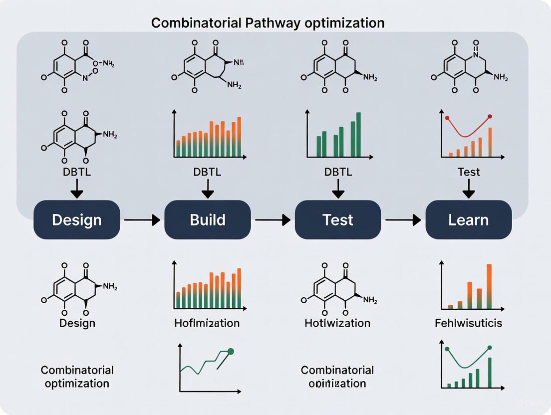
Workflow Visualization: DBTL Cycle
The following diagram illustrates the iterative, interconnected nature of the DBTL cycle and the key activities within each phase.
Advanced DBTL Paradigm: The LDBT Cycle and Machine Learning Integration
Recent advances are reshaping the traditional DBTL cycle. The integration of Machine Learning (ML) is so transformative that a new paradigm, the LDBT cycle (Learn-Design-Build-Test), has been proposed, where Learning precedes Design [7]. In this model, pre-trained ML models on vast biological datasets enable zero-shot predictions—generating functional designs without additional experimental training data [7]. This approach leverages powerful computational tools like protein language models (e.g., ESM, ProGen) and structure-based design tools (e.g., ProteinMPNN, MutCompute) to create highly optimized initial designs, potentially reducing the need for multiple iterative cycles [7].
Application Notes and Protocols for Combinatorial Pathway Optimization
Case Study: Automated DBTL for Flavonoid Production inE. coli
An automated DBTL pipeline was successfully applied to optimize a (2S)-pinocembrin biosynthetic pathway in E. coli, resulting in a 500-fold improvement in production titer, reaching 88 mg L⁻¹ [3]. The pathway consisted of four enzymes (PAL, CHS, CHI, 4CL) converting L-phenylalanine to pinocembrin.
Table 1: Key Experimental Results from Iterative DBTL Cycles for Pinocembrin Production
| DBTL Cycle | Number of Constructs | Design of Experiments Compression | Pinocembrin Titer Range (mg L⁻¹) | Key Learning |
|---|---|---|---|---|
| Cycle 1 | 16 | 162:1 (from 2592) | 0.002 – 0.14 | Vector copy number had the strongest positive effect (P = 2.00 × 10⁻⁸); CHI promoter strength also highly significant (P = 1.07 × 10⁻⁷). |
| Cycle 2 | 24 | Focused library based on Cycle 1 learning | Up to 88 mg L⁻¹ | Application of learned constraints (high copy number, strategic gene order) led to a 500-fold increase over the best initial construct. |
Detailed Protocol: Automated DBTL for Pathway Optimization
I. Design Phase Protocol
- Pathway Selection: Use RetroPath [3] to design the heterologous pathway from a defined starting metabolite (e.g., L-phenylalanine) to the target compound (e.g., pinocembrin).
- Enzyme Selection: Employ Selenzyme [3] to select candidate enzyme sequences for each reaction step.
- Combinatorial Library Design: Use software like PartsGenie [3] to design a library of genetic constructs, varying parameters such as:
- Vector backbone and copy number (e.g., ColE1 [high], p15a [medium], pSC101 [low]).
- Promoter strength (e.g., strong [Ptrc], weak [PlacUV5]).
- Gene order permutations within an operon.
- Library Compression: Apply Design of Experiments (DoE) based on orthogonal arrays to reduce the combinatorial library to a tractable number of representative constructs for building and testing [3].
II. Build Phase Protocol
- DNA Synthesis: Order designed gene sequences from commercial vendors [3].
- Automated DNA Assembly:
- Prepare DNA parts via PCR.
- Use a liquid-handling robot to set up Ligase Cycling Reaction (LCR) assembly reactions according to automated worklists generated by design software [3].
- Transformation and Quality Control:
- Transform LCR reactions into E. coli cloning strain (e.g., DH5α).
- Perform high-throughput plasmid purification from candidate clones.
- Verify constructs by restriction digest and capillary electrophoresis, followed by sequence verification [3].
III. Test Phase Protocol
- Strain Cultivation:
- Introduce verified constructs into the production chassis (e.g., E. coli DH5α).
- Perform automated cultivation in 96-deepwell plates using defined media and induction protocols [3].
- Metabolite Extraction: Use an automated liquid handler to extract metabolites from culture samples.
- Quantitative Analysis:
- Analyze samples using fast UPLC-MS/MS with high mass resolution.
- Quantify target product (pinocembrin) and key intermediates (e.g., cinnamic acid) by comparison to authentic standards [3].
- Use custom scripts (e.g., in R) for automated data extraction and processing.
IV. Learn Phase Protocol
- Statistical Analysis: Perform analysis of variance (ANOVA) to identify the impact of each design factor (e.g., copy number, promoter strength, gene order) on production titers [3].
- Modeling: Apply machine learning (e.g., linear models, random forest) to the dataset to build a predictive model of pathway performance [4].
- Design Refinement: Use the model and statistical insights to define constraints and priorities for the next design cycle, focusing on the most impactful parameters [3].
The Scientist's Toolkit: Key Research Reagent Solutions
Table 2: Essential Research Reagents and Tools for DBTL Cycles
| Item Name | Function/Application | Example Use Case |
|---|---|---|
| RetroPath [3] | Computational tool for automated metabolic pathway design. | Designing a novel pathway from a substrate to a target fine chemical. |
| Selenzyme [3] | Enzyme selection platform for choosing candidate sequences for pathway steps. | Selecting the most suitable 4-coumarate:CoA ligase (4CL) for a flavonoid pathway. |
| PartsGenie [3] | Software for designing reusable DNA parts with optimized RBS and coding sequences. | Designing a library of bicistronic constructs for RBS engineering in a dopamine pathway [8]. |
| Ligase Cycling Reaction (LCR) [3] | High-efficiency, automated DNA assembly method. | Assembling a combinatorial library of pathway variants into a plasmid backbone. |
| Cell-Free Protein Synthesis (CFPS) Systems [7] | Crude lysate or purified system for rapid in vitro transcription and translation. | Ultra-high-throughput prototyping of enzyme variants without cellular transformation [7]. |
| UTR Designer [8] | Tool for modulating Ribosome Binding Site (RBS) sequences to fine-tune translation. | Systematically varying the expression level of a pathway enzyme to balance flux. |
| JBEI-ICE Repository [3] | Open-source biological data management platform (jbe-ice.org). | Cataloging and tracking all designed DNA parts, plasmids, and associated metadata. |
The Challenge of Combinatorial Explosions in Metabolic Engineering and Drug Discovery
A considerable number of areas of bioscience, including gene and drug discovery and metabolic engineering, are best viewed as combinatorial optimization problems representing large search spaces of possible solutions populated by a much smaller number of optimal solutions [9]. The term "combinatorial explosion" describes the core challenge: the number of possible permutations in a system increases exponentially with the number of variables involved [10] [9]. In metabolic engineering, this manifests when optimizing multi-enzyme pathways, where testing all combinations of gene homologs, expression levels, and regulatory elements becomes experimentally intractable [10] [11]. Similarly, in drug discovery, screening all possible multi-drug combinations at varying doses from a library of candidate compounds is functionally impossible due to the astronomical number of possibilities [12].
This combinatorial explosion renders full factorial searches infeasible, forcing researchers to rely on sophisticated heuristic methods to identify "good enough" solutions without exhaustively testing every possibility [10] [9]. The fundamental problem is NP-hard, meaning the computational effort required for a definitive solution grows at a non-polynomial rate, quickly surpassing practical limits [9]. Addressing this challenge requires integrated strategies that combine smart experimental design with computational guidance to navigate the vast search spaces efficiently.
Table 1: Examples of Combinatorial Problem Scaling in Biology
| System Variables | Number of Components | Possible Combinations | Reference |
|---|---|---|---|
| Protein Engineering (300 aa) | 3 amino acid changes | ~30 billion | [9] |
| Metabolic Engineering | 6 enzymes with 5 variants each | 15,625 (5⁶) | [10] |
| Drug Screening | 4 drugs from 100 candidates | 3.9 million | [12] |
| DNA Aptamer (30mer) | 4 bases at 30 positions | 1.2 x 10¹⁸ (4³⁰) | [9] |
Application Notes: Metabolic Engineering
The Core Problem in Pathway Optimization
In metabolic engineering, combinatorial explosion arises when attempting to balance flux through heterologous pathways comprising multiple enzymatic steps [10]. Installing efficient pathways based purely on forward design rules remains infeasible due to insufficient a priori knowledge of pathway kinetics and intricate orchestration within cellular metabolism [10]. Traditional sequential optimization methods, which identify and remove major bottlenecks one at a time, often fail to identify globally optimal solutions because they neglect holistic interactions within the pathway and with host metabolism [10]. This limitation has driven the development of combinatorial pathway optimization approaches that create variant libraries where several pathway elements are diversified simultaneously [10] [11].
Key Diversification Strategies
Combinatorial optimization in metabolic engineering employs three primary diversification strategies, which can be used independently or in combination [10]:
Variation of Coding Sequences: This strategy employs different structural or functional gene homologs known (or suspected) to catalyze the respective reaction steps. In the absence of suitable candidates, metagenomic libraries can be exploited to identify appropriate biocatalysts [10]. For example, this approach was successfully used to graft xylose utilization into Saccharomyces cerevisiae [10].
Engineering of Expression Levels: Fine-tuning relative and absolute expression levels of involved genes is crucial for setting up a balanced pathway with high flux toward the desired product. This can be achieved by varying gene dosage through plasmid copy number or genomic integration sites, engineering transcription using promoter and terminator libraries, and modulating translation through ribosomal binding site (RBS) engineering [10] [11].
Combined and Integrated Approaches: The most powerful implementations simultaneously integrate different methods for diversity creation. For example, combinatorial refactoring of a 16-gene nitrogen fixation pathway from Klebsiella oxytoca into a E. coli host involved varying copy number, ribosome binding sites, and operon configurations, leading to a remarkable 50-fold improvement in ammonia production [10].
Protocol: Combinatorial Pathway Library Construction
Title: Modular Cloning for Combinatorial Pathway Assembly Application: Rapid generation of genetic diversity for metabolic pathway optimization Principle: Golden Gate and related DNA assembly methods utilize Type IIS restriction enzymes that cut outside their recognition sites, enabling seamless, directional, and simultaneous assembly of multiple DNA parts in a single reaction [13].
Table 2: Key Research Reagent Solutions for Combinatorial Pathway Engineering
| Reagent/Method | Function | Key Features |
|---|---|---|
| Type IIS Restriction Enzymes (e.g., BsaI) | Foundation of modular cloning systems; cut outside recognition sites | Creates unique, sequence-independent overhangs for seamless assembly |
| Golden Gate Assembly | Standardized framework for combinatorial part assembly | Modular, hierarchical; enables rapid variant generation |
| MoClo Toolkit | Standardized genetic part collections | Enables one-pot assembly of transcriptional units from promoters, CDS, terminators |
| Ribosome Binding Site (RBS) Libraries | Translation modulation | Varies protein expression levels without transcriptional changes |
| CRISPR/Cas9 Systems | Multiplex genome editing | Enables precise, simultaneous integration of pathway variants at genomic loci |
Materials:
- DNA parts library (promoters, RBS, coding sequences, terminators)
- Type IIS restriction enzyme (e.g., BsaI-HFv2)
- T4 DNA Ligase and buffer
- Thermocycler
- Competent E. coli cells
- Selection plates with appropriate antibiotics
Procedure:
- Library Design: Select DNA parts from standardized toolkits (e.g., MoClo). Design assembly using 4-bp overhangs that define part position and orientation [13].
- One-Pot Assembly Reaction:
- Combine approximately 50-100 ng of each DNA part
- Add 1.5 µL of BsaI-HFv2 (10 U/µL)
- Add 1 µL of T4 DNA Ligase (400 U/µL)
- Add 5 µL of 10X T4 DNA Ligase Buffer
- Adjust total volume to 50 µL with nuclease-free water
- Thermocycling: Program thermocycler: 25 cycles of (37°C for 3 minutes + 16°C for 4 minutes), then 50°C for 5 minutes, and 80°C for 10 minutes [13].
- Transformation: Transform 5 µL of assembly reaction into competent E. coli cells, plate on selective media, and incubate overnight.
- Screening/Selection: Pick colonies for screening or apply appropriate selection pressure to identify functional constructs.
Visualization: Combinatorial Pathway Optimization Workflow
Application Notes: Drug Discovery
The Combinatorial Therapy Challenge
In drug discovery, combinatorial explosion becomes problematic when seeking optimal multi-drug therapies [12]. While multidrug combination therapies often show better results than monotherapies against complex diseases, the number of possible combinations is staggering [12]. For example, a chemotherapy regimen comprising four drugs chosen from a library of 100 clinically used compounds, with three different doses possible for each drug, creates at least 3.2 × 10⁹ possibilities [12]. Conventional experimental platforms can typically test no more than 1000 combinations, covering only 0.00005% of this search space [12]. This massive discrepancy necessitates highly efficient and systematic optimization strategies.
Phenotype-Driven Optimization Approaches
The phenotype-driven medicine concept associates combinatorial drug therapy with systems engineering and optimization theories [12]. This approach considers the biological system as an open system and optimizes drug combinations as system inputs based on phenotypic outputs according to the formula:
Xopt = argmaxX E = argmax_X f(X)
where X is the drug combination input, E is the efficacy output (any measurable parameter), f is the function relation between drug doses and efficacy, and X_opt is the optimal combination [12]. This framework has introduced powerful approaches and tools to drug combination optimization, moving beyond the limitations of target-driven discovery.
Advanced Screening Platforms
Innovative laboratory platforms have been developed to enhance screening throughput and efficiency:
- Droplet Microfluidics: These systems enable high-throughput screening by encapsulating single cells or populations in nanoliter droplets along with specific drug combinations, allowing massive parallelization of experiments [12].
- Mass-Activated Droplet Sorting (MADS): This technology enables high-throughput screening of enzymatic reactions at nanoliter scale, combining the advantages of droplet microfluidics with sensitive mass spectrometric detection [12].
- 3D Tissue Models: Advanced in vitro systems including organoids, spheroids, and organ-on-a-chip platforms provide more physiologically relevant screening environments that better predict clinical efficacy [12].
Protocol: High-Throughput Combinatorial Drug Screening
Title: Droplet Microfluidic Screening for Drug Combination Discovery Application: Identification of synergistic drug combinations against cancer cell lines Principle: Nanoliter droplet encapsulation of cells with precise drug combinations enables massive parallel screening while conserving reagents and cells [12].
Materials:
- Drug compound library (prepared as concentrated stocks)
- Target cell line (e.g., cancer cells)
- Droplet microfluidics device (commercial or custom-fabricated)
- Fluorescent viability dyes (e.g., Calcein AM for live cells, Propidium Iodide for dead cells)
- Droplet generation oil and surfactants
- Flow cytometer or droplet sorter
Procedure:
- Drug Preparation: Prepare drug combinations in source plates using automated liquid handling systems. Create serial dilutions for dose-response studies.
- Cell Preparation: Harvest and resuspend cells in appropriate medium at optimized density (typically 10⁶ cells/mL).
- Droplet Generation:
- Load drug combinations and cell suspension into separate syringes
- Co-flow through microfluidic device to generate monodisperse droplets containing single cells with specific drug combinations
- Collect droplets in incubation chambers
- Incubation: Incude droplets at 37°C, 5% CO₂ for 48-72 hours to allow treatment effects to manifest.
- Viability Staining: Inject viability staining solutions into droplet stream using additional microfluidic inlets.
- Analysis and Sorting:
- Flow droplets through detection system measuring fluorescence signals
- Identify droplets containing viable cells based on fluorescence patterns
- Sort droplets containing promising drug combinations for further analysis
- Hit Validation: Break sorted droplets, recover cells, and validate hits in conventional well-plate assays.
Visualization: Combinatorial Drug Screening & Optimization
Computational Strategies to Counter Combinatorial Explosion
Heuristic Optimization Algorithms
Heuristic methods are essential for navigating combinatorial landscapes efficiently [9]. Several computational approaches have shown particular promise:
Evolutionary Computation: These algorithms maintain a population of candidate solutions that undergo selection, recombination, and mutation in cycles that mimic natural evolution [9]. The field that has been explicit in viewing scientific problem-solving as combinatorial optimization is evolutionary computing, where candidate solutions exhibit a level of "fitness" determined by the experimenter [9].
Active Learning: These algorithms use existing knowledge to determine the "best" experiment to do next, effectively modeling combinatorial landscapes in silico to guide experimental design [9]. By focusing experimental effort on the most promising regions of the search space, active learning dramatically reduces the number of experiments needed to find optimal solutions.
Machine Learning Integration: As the fields of combinatorial chemistry and computational chemistry have matured, combining them has led to higher hit rates [14]. It is more cost-effective to design and screen virtual chemical libraries in silico to define subsets of the chemical space likely to contain hits before actual synthesis and screening [14].
Protocol: Active Learning for Combinatorial Optimization
Title: Bayesian Optimization for Efficient Experimental Design Application: Guiding combinatorial library screening to maximize information gain Principle: Active learning algorithms select the most informative experiments to perform next based on previous results and uncertainty estimates, dramatically reducing the experimental burden [9].
Materials:
- Initial combinatorial library (pathway variants or drug combinations)
- High-throughput screening data from initial library
- Bayesian optimization software (e.g., GPyOpt, Dragonfly)
- Computational resources (workstation or cluster)
Procedure:
- Initial Screening: Screen a diverse but manageable subset (e.g., 5-10%) of the combinatorial library to generate initial training data.
- Model Training:
- Define objective function (e.g., product titer, cell viability)
- Train Gaussian process model on initial data to build surrogate model of the search space
- Quantize uncertainty estimates across unsampled regions
- Acquisition Function Optimization:
- Calculate acquisition function values (e.g., Expected Improvement, Upper Confidence Bound) for all unsampled combinations
- Select top candidates that balance exploration (high uncertainty regions) and exploitation (high predicted performance)
- Iterative Experimental Cycles:
- Experimentally test selected candidates from Step 3
- Update model with new experimental results
- Repeat selection process until performance plateaus or resources are exhausted
- Validation: Confirm optimal candidates identified through the process in biological replicates.
Table 3: Computational Approaches to Combat Combinatorial Explosion
| Method | Principle | Applications | Advantages |
|---|---|---|---|
| Active Learning | Selects most informative experiments based on previous results and model uncertainty | Pathway balancing, drug combination optimization | Reduces experimental burden by 10-100x |
| Evolutionary Algorithms | Mimics natural selection with populations of candidate solutions | Protein engineering, host optimization | Effective on rugged, non-linear landscapes |
| Bayesian Optimization | Builds probabilistic surrogate models of search space | Dose optimization, metabolic engineering | Handles noise and uncertainty effectively |
| PDGrapher (Graph Neural Networks) | Solves inverse problem of finding perturbations for desired state | Target identification, drug discovery | Direct prediction without exhaustive search [15] |
Integration in the Design-Build-Test-Learn Cycle
The most effective strategy for managing combinatorial explosion involves tight integration of combinatorial approaches within the Design-Build-Test-Learn (DBTL) framework [10] [11]. Each phase of the cycle contributes to progressively refining the search space:
Design Phase: Computational tools help design focused libraries that maximize diversity while minimizing redundancy. For metabolic engineering, this includes tools for enzyme selection, codon optimization, and expression balancing [13]. For drug discovery, in silico screening and virtual library design prioritize the most promising regions of chemical space [14].
Build Phase: Advanced DNA assembly methods [13] and combinatorial chemistry techniques [14] enable rapid construction of variant libraries. Modular cloning systems and DNA-encoded libraries have been particularly transformative in increasing construction efficiency.
Test Phase: High-throughput screening technologies including biosensors [11], droplet microfluidics [12], and advanced cytometry enable rapid evaluation of combinatorial libraries at unprecedented scale.
Learn Phase: Data from screening feeds back into computational models, refining understanding of the system and guiding the next Design phase. Machine learning methods excel at extracting complex patterns from high-dimensional combinatorial screening data [11] [15].
This iterative DBTL framework, enhanced by combinatorial methods and computational guidance, represents the most powerful approach to navigating the challenge of combinatorial explosions in metabolic engineering and drug discovery.
In the context of combinatorial pathway optimization using Design-Build-Test-Learn (DBTL) cycles, the accurate quantification of drug interaction effects is paramount for making informed decisions in subsequent design iterations. The primary goal of combining drugs is to achieve a synergistic effect, where the combined therapeutic impact is greater than the expected additive effect of the individual drugs. This allows for dosage reduction, decreased toxicity, and potentially overcoming drug resistance [16]. Two established reference models, Bliss Independence and the Combination Index (Chou-Talalay method), provide distinct mathematical frameworks for defining and quantifying these interactions [17]. While Bliss Independence operates on a probabilistic framework assuming drugs act independently through different pathways, the Combination Index is derived from the mass-action law principle and can be applied regardless of the drugs' mechanisms of action [18] [19]. This application note details the protocols for both methods, enabling researchers to robustly quantify drug synergy and antagonism, thereby providing critical, data-driven learning for optimizing therapeutic combinations in DBTL cycles.
Theoretical Foundations and Quantitative Comparison
Table 1: Core Principles of Bliss Independence and Combination Index Models
| Feature | Bliss Independence Model | Combination Index (Chou-Talalay) Model |
|---|---|---|
| Fundamental Principle | Probabilistic independence; drugs act on different pathways without interacting [17] [20]. | Mass-action law; dose-effect equivalence derived from enzyme kinetics [18] [19]. |
| Definition of Additivity (No Interaction) | Observed combination response equals the predicted response: (Yc = YA + YB - YA Y_B) [21] [17]. | Combination Index equals 1: (CI = \frac{dA}{D{A}} + \frac{dB}{D{B}} + \frac{dA dB}{D{A}D{B}} = 1) [21] [18]. |
| Definition of Synergism | Observed combination response greater than the Bliss-predicted response ((Yc > Yp)) [22]. | Combination Index less than 1 (CI < 1) [18] [19]. |
| Definition of Antagonism | Observed combination response less than the Bliss-predicted response ((Yc < Yp)) [22]. | Combination Index greater than 1 (CI > 1) [18] [19]. |
| Typical Application | Drugs with different mechanisms of action (mutually non-exclusive) [21]. | Applicable regardless of mechanism; can be used for both similar and different modes of action [18]. |
| Key Equation | (Yp = YA + YB - YA Y_B) (for inhibition/response) [17]. | (CI = \frac{dA}{D{A}} + \frac{dB}{D{B}}) (for mutually exclusive drugs) or (CI = \frac{dA}{D{A}} + \frac{dB}{D{B}} + \frac{dA dB}{D{A}D{B}}) (for mutually non-exclusive drugs) [21] [18]. |
The selection between Bliss Independence and the Combination Index often depends on the scientific question and the assumed mechanism of action. Bliss Independence is most appropriate when two drugs are believed to target different biological pathways and are mutually non-exclusive [21]. In contrast, the Chou-Talalay Combination Index method is a more general framework based on the median-effect principle, which is derived from the mass-action law [18] [19]. It does not require a priori knowledge of the drugs' mechanisms, as it can model both mutually exclusive and non-exclusive interactions [18]. A critical advancement in the application of Bliss Independence is the development of a two-stage response surface model, which allows for statistical testing of synergism across all tested dose combinations, reducing the risk of false-positive claims that can arise from simply comparing observed and predicted values without accounting for variability [21] [22].
Experimental Protocols
Protocol 1: Experimental Design and Viability Assay for Combination Screening
This protocol outlines the steps for designing and executing a drug combination experiment, from plate layout to data acquisition, which serves as the "Test" phase in a DBTL cycle.
Research Reagent Solutions:
- Cell Line: Select a relevant cancer cell line (e.g., LN229 glioblastoma [21] or MX-1 breast cancer [18]).
- Drugs: Gamitrinib (Hsp90 inhibitor) and a PI3K pathway kinase inhibitor [21], or Fludelone and Panaxytriol [18].
- Controls: Positive control (e.g., 10 μM Doxorubicin for 100% inhibition) and negative control (e.g., 0.2% DMSO for 0% inhibition) [21].
- Viability Assay Reagent: Fluorescent dye (e.g., for cell viability) or XTT assay kit [18].
Procedure:
- Plate Map Design: Utilize a matrix design (e.g., 7x7). The first block should include single-agent doses for Drug A (e.g., Gamitrinib) along one axis and single-agent doses for Drug B (e.g., a PI3K inhibitor) along the other. The inner cells of the matrix represent combination doses [21].
- Drug Dilution: Prepare a 1:3 serial dilution series for each drug, with the highest concentration typically in the micromolar range (e.g., 2.00 μM) and the lowest in the nanomolar range (e.g., 0.008 μM) [21].
- Cell Plating and Treatment: Plate cancer cells in a 384-well format. Treat cells with the single agents and combinations according to the plate map for a specified duration (e.g., 18 h at 37°C) [21].
- Viability Measurement: Add fluorescence or XTT viability reagent to the wells and incubate according to manufacturer specifications. Measure the fluorescence or absorbance intensity using a plate reader [21] [18].
- Data Normalization: Calculate the fractional viability for each well by normalizing its readout to the aggregate averages of the positive control (0% viability) and negative control (100% viability) wells. The fractional growth inhibition rate (the response, (Y)) is then calculated as (1 - \text{viability}) [21].
Protocol 2: Data Analysis using the Bliss Independence Model
This protocol details the statistical analysis of combination data under the Bliss independence assumption, transforming raw data into a quantitative assessment of synergy.
Procedure:
- Calculate Bliss Prediction: For each combination dose ((dA, dB)), calculate the predicted inhibition rate ((Yp)) under the assumption of independence using the formula: (Yp = YA + YB - YA \cdot YB), where (YA) and (YB) are the observed inhibition rates for drug A and drug B alone at doses (dA) and (dB), respectively [21] [17].
- Compute Excess Over Bliss: For each combination, subtract the predicted response from the observed combination response ((Yc)): (\text{Excess} = Yc - Y_p). A positive excess indicates synergism, while a negative value indicates antagonism [21].
- Statistical Modeling (Two-Stage Model): To avoid false positives and account for data variability, fit a two-stage response surface model [21] [22].
- Stage 1: Fit non-linear dose-response curves (e.g., sigmoidal Emax model) to the single-agent data for each drug to estimate their parameters.
- Stage 2: Using the parameters from Stage 1, fit a global model to the combination data to estimate an overall interaction index (τ) with a 95% confidence interval. An index significantly less than 0 indicates overall synergism [21].
- Visualization: Generate a surface plot or heat map showing the "excess over Bliss" across the entire dose matrix to visualize regions of synergy and antagonism [21].
Protocol 3: Data Analysis using the Chou-Talalay Combination Index Method
This protocol describes the use of the median-effect equation and Combination Index to quantify drug interactions, a method widely adopted in the field.
Procedure:
- Median-Effect Plot: For each single agent and the combination at a fixed ratio, calculate the dose and effect. Plot (\log \left( \frac{fa}{fu} \right)) vs. (\log(\text{dose})), where (fa) is the fraction affected and (fu) is the fraction unaffected ( (fu = 1 - fa) ). This is the median-effect plot [18] [17].
- Determine Median-Effect Parameters: Fit a linear regression to the median-effect plot. The slope of the line is (m) (the shape parameter of the dose-effect curve), and the x-intercept is (\log(Dm)), where (Dm) is the median-effect dose (e.g., IC50 or GI50) [18].
- Calculate Combination Index (CI): For a given combination effect level (fa), use the equation for mutually non-exclusive drugs: ( CI = \frac{(dA)}{(D{m,A}) \left( \frac{fa}{1-fa} \right)^{1/mA}} + \frac{(dB)}{(D{m,B}) \left( \frac{fa}{1-fa} \right)^{1/mB}} + \frac{(dA)(dB)}{(D{m,A}) \left( \frac{fa}{1-fa} \right)^{1/mA} (D{m,B}) \left( \frac{fa}{1-fa} \right)^{1/mB}} ) where (dA) and (dB) are the doses of drug A and B in combination that produce effect (fa), and (D{m,A}) and (D{m,B}) are the doses of each drug alone that produce the same effect [18].
- Interpretation: A CI < 1 indicates synergism, CI = 1 indicates an additive effect, and CI > 1 indicates antagonism [18] [19].
- Software-Assisted Analysis: Input the dose-response data for single agents and the combination into software like CompuSyn to automatically generate the median-effect plots, CI values, Fa-CI plots, and isobolograms [18].
Integration with DBTL Cycles & Visualization
The quantitative outputs from these synergy models are the cornerstone of the "Learn" phase in a DBTL cycle for combinatorial pathway optimization. The results directly inform the next "Design" phase, guiding whether to pursue a specific drug pair, optimize the ratio of compounds, or investigate the underlying biological pathways further.
Diagram 1: The DBTL cycle for combinatorial drug optimization, highlighting the integration of Bliss and Combination Index (CI) models within the "Learn" phase to inform subsequent design iterations.
Table 2: Interpreting Model Outputs for DBTL Cycle Decisions
| Model Output | Observation | DBTL Cycle Decision & Action |
|---|---|---|
| Bliss: Significant negative τ [21]CI: Consistent CI < 0.9 [18] | Strong, overall synergism | Proceed & Optimize: Advance the drug combination to the next DBTL cycle. Actions may include refining the dose ratio, testing in more complex models (e.g., 3D cultures, in vivo), or scaling up synthesis. |
| Bliss: τ not significantCI: CI ≈ 1 | Additive effect | Re-design or Terminate: The combination offers no superior effect. Consider re-designing the combination with different drugs or mechanisms of action, or terminate the project to save resources. |
| Bliss: Significant positive τ [21]CI: CI > 1.1 [18] | Antagonism | Terminate or Investigate: The combination is counterproductive. The combination should be abandoned unless the antagonistic effect is desired for a specific context (e.g., reducing toxicity of one drug [18]). |
| Bliss: Synergy only at high dosesCI: Synergy only at high Fa | Dose-dependent synergism | Re-design & Refine: The therapeutic window may be narrow. Re-design the experiment to focus on the synergistic dose range and ratio in the next cycle. |
The rigorous application of both Bliss Independence and Combination Index models provides a powerful, quantitative framework for evaluating drug combinations within combinatorial pathway optimization research. By implementing the detailed experimental and analytical protocols outlined in this note, researchers can consistently transition from raw viability data to statistically robust conclusions regarding synergism and antagonism. This quantitative learning is essential for guiding intelligent decisions in iterative DBTL cycles, ultimately accelerating the development of effective, multi-target therapeutic strategies with the potential to reduce toxicity and overcome drug resistance.
The Design-Build-Test-Learn (DBTL) cycle is a foundational framework in synthetic biology and metabolic engineering for developing efficient microbial cell factories [5]. The integration of multi-omics data—genomics, transcriptomics, and proteomics—has revolutionized this cycle by providing deep, system-wide molecular insights that inform each stage. This integration moves pathway design beyond static genomic information to incorporate dynamic functional data, enabling more predictive and efficient engineering of biological systems [23] [24]. The application of multi-omics within DBTL cycles has been particularly transformative for combinatorial pathway optimization, where understanding interactions between multiple genetic modifications is crucial for maximizing product yields and cellular fitness [5].
Table: Multi-Omics Data Types and Their Roles in Pathway Design
| Omics Layer | Data Content | Role in Pathway Design |
|---|---|---|
| Genomics | DNA sequence, mutations, copy number variations | Identifies target genes for modification, reveals structural variants, provides context for host engineering |
| Transcriptomics | RNA expression levels, transcript sequences | Reveals gene expression dynamics, identifies regulatory elements, monitors cellular response to pathway engineering |
| Proteomics | Protein abundance, post-translational modifications, protein-protein interactions | Confirms functional enzyme levels, identifies bottlenecks in metabolic flux, reveals regulatory mechanisms |
Computational Frameworks for Multi-Omics Integration
Effective integration of multi-omics data requires sophisticated computational frameworks that can handle the heterogeneity, scale, and complexity of diverse molecular datasets. Several approaches have emerged to address these challenges.
The SynOmics framework represents a significant advancement through its use of graph convolutional networks to model both within- and cross-omics dependencies [25]. Unlike traditional early or late integration strategies, SynOmics adopts a parallel learning strategy that processes feature-level interactions at each model layer, enabling more nuanced capture of cross-omics relationships. This approach constructs omics networks in feature space, incorporating both omics-specific networks and cross-omics bipartite networks to simultaneously learn intra-omics and inter-omics relationships [25]. Experimental results demonstrate that SynOmics consistently outperforms state-of-the-art multi-omics integration methods across various biomedical classification tasks, highlighting its potential for enhancing pathway design predictions [25].
For visualization and exploration of integrated multi-omics data, tools like the expanded Cellular Overview in Pathway Tools (PTools) enable researchers to simultaneously visualize up to four types of omics data on organism-scale metabolic network diagrams [26]. This tool maps different omics datasets to distinct visual channels—reaction arrow color and thickness, plus metabolite node color and thickness—allowing intuitive interpretation of complex relationships across molecular layers. The system supports semantic zooming for detailed exploration and can animate datasets with multiple time points to reveal dynamic patterns [26].
Table: Benchmarking Multi-Omics Study Design Factors for Robust Analysis
| Factor Category | Specific Factor | Recommended Guideline | Impact on Analysis |
|---|---|---|---|
| Computational | Sample Size | ≥26 samples per class | Ensures statistical power and reliability |
| Computational | Feature Selection | <10% of omics features selected | Improves clustering performance by 34% |
| Computational | Class Balance | Under 3:1 ratio between classes | Prevents algorithmic bias toward majority class |
| Computational | Noise Characterization | Below 30% noise level | Maintains signal integrity and pattern recognition |
| Biological | Omics Combinations | GE + MI + CNV + ME | Optimal for cancer subtyping based on TCGA analysis |
Experimental Protocols for Multi-Omics Data Generation
Genomics and Transcriptomics Profiling
Protocol 1: Whole Genome Sequencing for Pathway Engineering
- DNA Extraction: Use high-quality extraction kits to obtain high-molecular-weight DNA from bacterial cultures (OD₆₀₀ ≈ 0.6-0.8)
- Library Preparation: Utilize Illumina-compatible library prep kits with fragmentation to 350-500bp following manufacturer protocols
- Sequencing: Run on Illumina NovaSeq X platform with 2×150bp paired-end reads, targeting 30-50x coverage
- Variant Calling: Process with DeepVariant for SNP and indel identification, using default parameters [23]
- Analysis: Map reads to reference genome using BWA-MEM, identify structural variants with Manta, and annotate with SNPEff
Protocol 2: RNA-Seq for Transcriptomic Profiling of Engineered Strains
- RNA Extraction: Harvest cells during mid-log phase, stabilize immediately in RNA-protect reagent, extract using column-based methods
- Quality Control: Verify RNA Integrity Number (RIN) >8.0 using Bioanalyzer
- Library Preparation: Deplete rRNA using specific probes, prepare stranded RNA-seq libraries with unique dual indexes
- Sequencing: Sequence on Illumina platform to depth of 20-30 million reads per sample
- Analysis: Align to reference genome with STAR, quantify gene expression with featureCounts, perform differential expression with DESeq2
Proteomics Analysis
Protocol 3: Mass Spectrometry-Based Proteomics for Pathway Flux Analysis
- Protein Extraction: Lyse cells in 8M urea buffer with protease inhibitors, sonicate on ice (3×10s pulses)
- Digestion: Reduce with 5mM DTT (30min, 37°C), alkylate with 15mM iodoacetamide (30min, dark), digest with trypsin (1:50 ratio, overnight, 37°C)
- Desalting: Desalt peptides using C18 stage tips, dry in vacuum concentrator
- LC-MS/MS Analysis: Reconstitute in 0.1% formic acid, separate on nano-LC system (75μm×25cm C18 column, 90min gradient), analyze on timsTOF Pro mass spectrometer in DIA mode
- Data Processing: Process using Spectronaut with default settings, quantify against organism-specific database
Protocol 4: Benchtop Protein Sequencing for Rapid Validation
- Sample Preparation: Digest proteins into peptides using Platinum Pro kit reagents following manufacturer's protocol [27]
- Chip Loading: Apply peptides to specialized sequencing chips containing millions of wells
- Sequencing: Run on Quantum-Si's Platinum Pro single-molecule protein sequencer with integrated analysis [27]
- Data Interpretation: Use proprietary software to identify amino acid sequences and post-translational modifications
Multi-Omics Visualization and Workflow Integration
Effective visualization is critical for interpreting multi-omics data within pathway design contexts. The following diagram illustrates the integration of multi-omics data into the DBTL cycle for combinatorial pathway optimization:
The integration of diverse omics data types requires specialized visualization approaches. The following diagram illustrates how different omics layers can be simultaneously visualized on metabolic pathway maps to inform design decisions:
The Scientist's Toolkit: Essential Research Reagents and Platforms
Table: Key Research Reagent Solutions for Multi-Omics Pathway Design
| Tool/Platform | Type | Primary Function | Application in Pathway Design |
|---|---|---|---|
| Illumina NovaSeq X | Sequencing Platform | High-throughput DNA/RNA sequencing | Whole genome sequencing of engineered strains, transcriptome profiling |
| SomaScan Platform | Proteomics Tool | Affinity-based protein quantification | Measuring pathway enzyme abundance in response to genetic modifications |
| Quantum-Si Platinum Pro | Protein Sequencer | Benchtop single-molecule protein sequencing | Validating enzyme sequences in engineered pathways [27] |
| Olink Explore HT | Proteomics Platform | Multiplex protein quantification | High-throughput verification of proteomic changes in engineered strains |
| Pathway Tools | Software Suite | Metabolic pathway analysis and visualization | Multi-omics data visualization on metabolic maps [26] |
| SynOmics | Computational Framework | Graph-based multi-omics integration | Modeling cross-omics dependencies in engineered pathways [25] |
| Ultima UG 100 | Sequencing System | High-throughput, cost-efficient sequencing | Large-scale validation of engineered pathway libraries |
The integration of genomics, transcriptomics, and proteomics data has fundamentally transformed pathway design within DBTL cycles, enabling more predictive and efficient engineering of biological systems. By leveraging computational frameworks like SynOmics for data integration [25], advanced visualization tools for interpretation [26], and high-throughput technologies for data generation [27], researchers can now navigate the complexity of biological systems with unprecedented precision. As these multi-omics approaches continue to mature alongside developments in AI and machine learning [23] [24], they promise to accelerate the design of optimized biological pathways for therapeutic development, sustainable manufacturing, and agricultural innovation.
Combinatorial optimization represents a paradigm shift in both cancer therapy and microbial metabolic engineering. The core principle involves the systematic testing of multiple factors simultaneously—be they drugs, genetic parts, or environmental conditions—to discover synergistic interactions that a sequential approach would likely miss. This methodology is formally structured within the Design-Build-Test-Learn (DBTL) cycle, a framework that accelerates the development of complex biological systems by iteratively refining hypotheses based on experimental data [8]. In oncology, this has evolved from the early use of single cytotoxic agents to sophisticated multi-drug regimens and conjugated combinations that target specific cancer pathways, dramatically improving patient survival [28] [29]. Similarly, in microbial engineering, combinatorial optimization of pathway genes, rather than sequential tuning, is crucial for breaking through production bottlenecks and achieving economically viable titers of valuable metabolites, from biofuels to pharmaceuticals [30] [31]. The following sections detail the application notes and experimental protocols that underpin this powerful approach.
Application Notes: Anti-Cancer Drug Cocktails
The development of combination cancer therapy began with the recognition that single-agent treatments often yielded only transient benefits, followed by disease recurrence due to drug resistance. The shift to combination regimens was a pivotal advancement in clinical oncology [28].
Historical Evolution and Key Principles
The following table summarizes the evolution of cancer chemotherapy, highlighting the key advancements and their impacts.
Table 1: Evolution of Cancer Chemotherapy Approaches
| Era | Therapeutic Approach | Key Examples | Impact and Limitations |
|---|---|---|---|
| 1940s-1950s | Single-agent cytotoxic therapy | Nitrogen mustards, Aminopterin | Demonstrated principle of chemical tumor control; transient responses, universal resistance, severe toxicity [28]. |
| 1960s-Present | Multi-drug combination cocktails | Combination regimens for childhood Acute Lymphoblastic Leukemia (ALL) | Overcame resistance, increased cure rates; severe, dose-limiting toxicities remained a major challenge [28]. |
| 2000s-Present | Targeted therapy & combination | Imatinib for CML, combinations of targeted drugs | Selective targeting of cancer-specific molecules; significantly reduced toxicity, high remission rates (e.g., CML survival from ~20% to >90%) [28]. |
| Present-Future | Conjugated drug combinations & novel modalities | Antibody-Drug Conjugates (ADCs), Bispecific T-cell engagers | Selective delivery of potent cytotoxins to tumor cells (ADCs); redirecting immune cells to tumors (bispecifics); improved therapeutic window [28] [32]. |
Recent Clinical Applications and FDA Approvals (2024-2025)
Recent FDA approvals exemplify the trend towards targeted, biomarker-driven combination strategies and improved drug delivery methods.
Table 2: Select Recent FDA Approvals in Oncology (2024-2025) Illustrating Combination and Delivery Strategies
| Drug (Brand Name) | Approval Date | Indication | Key Combinatorial or Delivery Insight |
|---|---|---|---|
| Dordaviprone (Modeyso) | Q3 2025 | H3 K27M-mutated diffuse midline glioma | First-in-class therapy with dual mechanism: inhibits D2/3 dopamine receptor and overactivates mitochondrial ClpP enzyme [32]. |
| Zongertinib (Hernexeos) | Q3 2025 | HER2-mutated non-small cell lung cancer (NSCLEX) | Oral tyrosine kinase inhibitor; effective against broader HER2 mutations than existing therapy; demonstrates a "very favorable safety profile" [32]. |
| Imlunestrant (Inluriyo) | Q3 2025 | ESR1-mutated, ER+/HER2- advanced breast cancer | A "pure" estrogen receptor (ER) blocker (SERD); effective alone and in combination with the CDK4/6 inhibitor abemaciclib [32]. |
| Linvoseltamab-gcpt (Lynozyfic) | Q3 2025 | Relapsed/refractory multiple myeloma | Bispecific T-cell engager; combinatorially targets BCMA on cancer cells and CD3 on T cells to engage immune system for tumor cell killing [32]. |
| Pembrolizumab (Keytruda) Subcutaneous | Q3 2025 | Multiple solid tumors | New delivery method (subcutaneous injection) for an existing drug, improving patient accessibility and convenience compared to intravenous infusion [32]. |
| Avutometinib + Defactinib (Co-Pack) | H1 2025 | KRAS-mutated recurrent ovarian cancer | Novel drug combination targeting KRAS-driven cancers, representing a new treatment option for a rare cancer [33]. |
Application Notes: Microbial Metabolite Production
Microbial cell factories are engineered to produce valuable secondary metabolites, which include many antibiotics, anticancer agents, and agrochemicals. The optimization of these pathways is a central challenge in metabolic engineering.
The Role of Secondary Metabolites and Optimization Challenge
Microbial secondary metabolites are non-essential molecules produced from intermediates of primary metabolism. They are a rich source of bioactivity. It is estimated that 45% of all bioactive microbial metabolites are produced by Actinomycetales, with the genus Streptomyces alone producing approximately 7,600 compounds [34]. Optimizing the production of these compounds requires balancing the expression of multiple pathway genes, as the abundance of one enzyme often becomes the limiting factor for the entire pathway's flux [30].
Quantitative Analysis of Combinatorial Pathway Optimization
The table below summarizes key results from studies that implemented combinatorial optimization using Design of Experiments (DoE) in microbial systems.
Table 3: Performance Gains from Combinatorial Pathway Optimization in Microbial Cell Factories
| Target Product | Host Organism | Number of Factors Optimized | Optimization Strategy | Resulting Improvement | Source |
|---|---|---|---|---|---|
| p-Coumaric Acid (pCA) | Saccharomyces cerevisiae | 6 genetic + 3 environmental | Two rounds of fractional factorial DoE | 168-fold variation in pCA titer; identified significant interaction between culture temperature and ARO4 gene expression [31]. | |
| Dopamine | Escherichia coli | 2 genes (HpaBC, Ddc) | Knowledge-driven DBTL cycle with high-throughput RBS engineering | Final titer of 69.03 ± 1.2 mg/L (34.34 ± 0.59 mg/g biomass), a 2.6 to 6.6-fold improvement over the state-of-the-art [8]. | |
| Curcuminoid Pathway Analysis | In silico kinetic model | 7 enzymes | Simulated full factorial (128 strains) vs. fractional factorial designs | Resolution IV designs provided the best trade-off, identifying optimal strains with fewer constructions while capturing interactions [30]. |
Experimental Protocols
Protocol 1: Combinatorial Optimization of a Microbial Pathway using Fractional Factorial Design
This protocol outlines the use of a Resolution IV fractional factorial design to optimize a multi-gene pathway in S. cerevisiae for p-coumaric acid production [31].
1. Design Phase
- Define Factors and Levels: Select the pathway genes to be optimized. For initial screening, choose two expression levels per gene (e.g., low and high, represented by weak and strong promoters).
- Select DoE Design: For 6 factors, a full factorial design would require 2^6 = 64 strains. A Resolution IV fractional factorial design can be generated using statistical software (e.g., the
FrF2package in R), requiring only 16-32 strains. This design confounds two-factor interactions with each other but allows clear identification of all main effects [30] [31]. - Strain Design Table: Create a table specifying the genetic construct for each strain to be built.
2. Build Phase
- Strain Construction: Use automated genetic engineering platforms (e.g., Golden Gate assembly followed by in vivo recombination in a Cas9-equipped host strain) to construct the library of yeast strains as per the design table [31].
- Culture Stock Preparation: Pick single colonies into 96-well plates containing solid growth medium with appropriate selection agents. Incubate at 30°C for 3 days and store correct strains at -80°C in 10% glycerol.
3. Test Phase
- Inoculation and Cultivation:
- Grow single colonies in 10 mL of rich medium (e.g., YPDA) in 50 mL tubes for 24 hours.
- Wash cultures and inoculate into defined minimal media with 20 g/L glucose in deep-well plates, to a starting OD specified by the experimental design.
- Vary other process factors as per the DoE (e.g., nitrogen source: ammonium sulfate vs. urea; pH buffered or not).
- Incubate with shaking at temperatures specified by the design (e.g., 20°C, 30°C) for a fixed period [31].
- Analytics: Measure the final optical density (OD) and the concentration of the target metabolite (e.g., p-coumaric acid) in the supernatant via High-Performance Liquid Chromatography (HPLC).
4. Learn Phase
- Statistical Analysis: Fit the production data to a linear model using ordinary least squares regression. The model will have the form:
y = β₀ + Σ(ME_i * F_i) + Σ(2FI_i:j * F_i * F_j)whereyis the product titer,β₀is the intercept,ME_iis the main effect of factor i, and2FI_i:jis the two-factor interaction between i and j [30]. - Analysis of Variance (ANOVA): Perform ANOVA to determine which main effects and interactions significantly influence production.
- Decision Making: Identify the most important factors and their optimal levels. Use these insights to design a subsequent DBTL cycle with a narrower focus or more levels for the critical factors.
Protocol 2: Knowledge-Driven DBTL Cycle for Dopamine Production in E. coli
This protocol leverages upstream in vitro experiments to inform the initial design of the in vivo DBTL cycle, accelerating strain optimization [8].
1. Design Phase
- In Vitro Pathway Analysis:
- Prepare crude cell lysates from an E. coli production host.
- Clone the pathway genes (e.g., hpaBC and ddc for dopamine) into individual plasmids under an inducible promoter (e.g., pJNTN system).
- In a cell-free reaction buffer containing substrates (L-tyrosine, cofactors FeCl₂, vitamin B6), test different relative expression levels by varying the plasmid ratios.
- Analyze L-DOPA and dopamine production to determine the optimal enzyme ratio for the pathway [8].
- In Vivo RBS Library Design: Based on the optimal ratio, design a library of bicistronic constructs for the two genes. Use RBS engineering to fine-tune the translation initiation rate (TIR) of the second gene (ddc) relative to the first (hpaBC). Design a series of RBS sequences with varying Shine-Dalgarno sequences to modulate strength without altering the coding sequence [8].
2. Build Phase
- Library Construction: Assemble the bicistronic construct with the variable RBS for ddc into a backbone plasmid. Use Golden Gate assembly or similar high-throughput methods.
- Strain Transformation: Transform the plasmid library into a genomically engineered E. coli host strain optimized for L-tyrosine overproduction (e.g., FUS4.T2 with TyrR depletion and feedback-resistant tyrA) [8].
3. Test Phase
- High-Throughput Screening:
- Grow transformants in 96-well plates containing minimal medium with appropriate inducers (e.g., 1 mM IPTG).
- After cultivation, measure biomass (OD) and dopamine production. Dopamine can be quantified via HPLC or, for initial screening, correlated with the formation of dark melanin-like pigments in alkaline conditions.
- Select the top-performing strains for validation in shake-flask cultures [8].
- Analytical Validation: Confirm dopamine titers in shake-flask supernatances using HPLC with standard calibration curves.
4. Learn Phase
- Correlation Analysis: Analyze the correlation between the designed RBS strength (e.g., predicted Gibbs free energy), the relative expression level of Ddc, and the final dopamine titer.
- Model Refinement: Update the model of the pathway to incorporate the learned relationship between RBS sequence, enzyme activity, and flux.
- Cycle Iteration: If the target titer is not met, initiate a new DBTL cycle, which could involve fine-tuning the first gene's expression, introducing additional genomic modifications, or optimizing process parameters like temperature and media composition.
Visualizing Workflows and Pathways
The DBTL Cycle for Combinatorial Optimization
Diagram Title: The Iterative DBTL Cycle
Dopamine Biosynthesis Pathway from L-Tyrosine
Diagram Title: Dopamine Biosynthesis Pathway
The Scientist's Toolkit: Essential Research Reagents and Materials
Table 4: Key Research Reagent Solutions for Combinatorial Optimization
| Reagent / Material | Function / Application | Example Use Case |
|---|---|---|
| Plasmid Systems (e.g., pET, pJNTN) | Storage and expression of heterologous genes; library construction. | Hosting genes hpaBC and ddc for dopamine production in E. coli [8]. |
| Promoter & RBS Library | Fine-tuning gene expression levels in a pathway. | Combinatorial optimization of 6 genes in S. cerevisiae using different promoters [31]; RBS engineering in E. coli [8]. |
| Cas9-integrated Host Strain | Enables precise genomic integration of pathway gene clusters. | S. cerevisiae host for efficient, standardized genomic integration of designed pathway constructs [31]. |
| DoE Software (e.g., R FrF2, JMP) | Generates efficient fractional factorial design matrices and analyzes results. | Creating a Resolution IV design for 7 factors to reduce the number of strains from 128 to a more manageable subset [30]. |
| Cell-Free Protein Synthesis (CFPS) System | In vitro testing of enzyme expression and pathway flux without cellular constraints. | Determining the optimal ratio of HpaBC to Ddc enzyme activity before in vivo strain building [8]. |
| HPLC / GC-MS Systems | Accurate quantification of target metabolite titers and analysis of metabolic profiles. | Measuring p-coumaric acid or dopamine concentrations in culture supernatants [31] [8]. |
Implementing DBTL: From AI-Driven Design to High-Throughput Building and Testing
The Design-Build-Test-Learn (DBTL) cycle is a foundational framework for modern combinatorial pathway optimization in drug development. Machine learning (ML) serves as the core "Learn" component, transforming experimental data into predictive models that guide subsequent "Design" phases, thereby creating an iterative, data-driven feedback loop. This accelerates the discovery of synergistic drug combinations and optimized therapeutic agents. Among the plethora of ML techniques, Gradient Boosting, Random Forests, and Deep Learning have emerged as particularly powerful for predictive modeling tasks. These methods excel at analyzing complex, high-dimensional biological data—including multi-omics profiles, chemical structures, and protein-protein interaction networks—to predict bioactivity, synergy, and other critical parameters. Their integration into DBTL cycles enables researchers to move beyond empirical trial-and-error, instead using computational predictions to prioritize the most promising experiments, significantly reducing development time and costs [35] [36].
The following table summarizes the core characteristics and applications of these key ML methods in the context of DBTL-driven research.
Table 1: Key Machine Learning Methods in Predictive Modeling for Drug Discovery
| Method | Core Principle | Key Advantages | Typical Applications in DBTL |
|---|---|---|---|
| Gradient Boosting | Sequentially builds an ensemble of weak prediction models (typically trees), where each new model corrects the errors of the previous one. | High predictive accuracy, robust handling of mixed data types, often wins data science competitions. | Building baseline predictive models for activity or toxicity; feature importance analysis to guide design [37] [38]. |
| Random Forests | An ensemble "bagging" method that constructs a multitude of decision trees at training time and outputs the mode (classification) or mean (prediction) of the individual trees. | Reduces overfitting, handles high-dimensional data well, provides intrinsic feature importance measures. | Initial screening of compound libraries; QSAR modeling; identifying critical genomic features [37] [39]. |
| Deep Learning (e.g., DeepSynergy) | Uses neural networks with many layers ("deep") to learn hierarchical representations and complex, non-linear patterns directly from raw or structured data. | State-of-the-art performance on large datasets; ability to automatically learn relevant features from complex inputs like graphs and multi-omics data. | Predicting novel synergistic drug combinations [37] [40]; integrating multi-omics data for patient-specific predictions [41]. |
Application Notes: ML for Drug Synergy Prediction
Predicting synergistic drug combinations is a central challenge in oncology and complex disease therapy, perfectly suited for ML-powered DBTL cycles. The following application notes detail the implementation and performance of specific deep learning models designed for this task.
Table 2: Comparison of Deep Learning Models for Drug Synergy Prediction
| Model Name | Input Data & Key Innovations | Reported Performance | Context in DBTL Cycle |
|---|---|---|---|
| DeepSynergy | Inputs: Chemical drug descriptors and genomic information (gene expression) of cancer cell lines.Innovation: One of the first deep learning models applied to large-scale drug synergy prediction; uses conical layers to model drug-cell line interactions [37] [38]. | - Mean Squared Error: Significantly outperformed other methods (7.2% improvement over second best).- Pearson Correlation: 0.73 for novel combinations within explored space.- Classification AUC: 0.90 for classifying synergistic combinations [37]. | Learn/Design: The model is trained on high-throughput screening data ("Test" phase) and used to predict and prioritize novel, untested drug-cell line combinations for the next "Design" and "Build" cycle. |
| AuDNNsynergy | Inputs: Multi-omics data (gene expression, copy number variation, mutation) from TCGA and chemical structure data.Innovation: Uses separate autoencoders for each omics data type to create compressed, informative representations of cell lines before feeding them into a deep neural network [41]. | - Outperformed four state-of-the-art approaches, including DeepSynergy, Gradient Boosting Machines, Random Forests, and Elastic Nets [41]. | Learn/Design: Enhances the "Learn" phase by integrating diverse data modalities, leading to more biologically informed predictions for designing new experiments. |
| MultiSyn | Inputs: Multi-omics data, protein-protein interaction (PPI) networks, and drug molecules decomposed into pharmacophore-containing fragments.Innovation: A semi-supervised graph neural network integrates PPI networks with multi-omics data for cell line representation. Uses a heterogeneous graph transformer to learn multi-view drug representations, improving interpretability [40]. | - Outperformed several classical and state-of-the-art baselines (e.g., DeepSynergy, DeepDDS).- Provides visualization of key substructures critical for synergy, enhancing mechanistic understanding [40]. | Learn/Design: Represents an advanced "Learn" phase that incorporates biological network context and pharmacophore information, yielding more accurate and interpretable predictions for the subsequent "Design" of optimized drug combinations and candidates. |
Experimental Protocols
This section provides detailed, step-by-step methodologies for implementing the machine learning workflows discussed, enabling researchers to integrate these protocols into their own DBTL cycles.
Protocol: Implementing a DeepSynergy-like Model for Synergy Prediction
This protocol outlines the procedure for developing a deep learning model to predict anti-cancer drug synergy, based on the architecture and methodology of DeepSynergy [37] [38].
I. Data Acquisition and Preprocessing
- Obtain Synergy Data: Acquire a large-scale drug combination screening dataset. Example: The O'Neil et al. dataset (23,062 samples, 38 drugs, 39 cell lines) used in the original DeepSynergy study [38].
- Collect Drug Features: For each drug, compute or retrieve molecular descriptors (e.g., molecular weight, logP) and fingerprint vectors (e.g., ECFP4) from chemical databases like PubChem or using toolkits like RDKit.
- Collect Cell Line Features: For each cancer cell line, download normalized gene expression profiles (e.g., RNA-Seq or microarray data) from repositories such as the Cancer Cell Line Encyclopedia (CCLE).
- Data Integration and Normalization: Merge the drug and cell line features with the synergy scores. Apply a robust normalization strategy (e.g., Z-score normalization) to all input features to account for data heterogeneity and improve model convergence.
II. Model Architecture and Training
- Input Layer: Create two separate input branches: one for the drug pair (concatenated features of both drugs) and one for the cell line genomic features.
- Hidden Layers:
- Utilize fully connected (dense) layers with non-linear activation functions (e.g., ReLU).
- Implement a specific architectural feature like "conical" layers, where the number of neurons decreases in subsequent layers, forcing the network to learn a compressed, meaningful representation of the input.
- Merge the drug and cell line pathways in the network to model their interaction.
- Output Layer: Use a single neuron with a linear activation function for regression, predicting the continuous synergy score.
- Training Procedure:
- Partitioning: Split the data into training, validation, and test sets. Use a cell-line-wise or drug-wise split to rigorously assess the model's ability to generalize to novel contexts.
- Loss Function: Use Mean Squared Error (MSE) as the loss function.
- Optimization: Train the model using a stochastic gradient descent optimizer (e.g., Adam) with early stopping based on the validation set performance to prevent overfitting.
III. Model Validation and Interpretation
- Performance Evaluation: Calculate the Mean Squared Error (MSE) and Pearson correlation coefficient between the measured and predicted synergy scores on the held-out test set.
- Benchmarking: Compare the model's performance against established baseline methods, such as Gradient Boosting Machines and Random Forests, to demonstrate its superiority.
- Analysis: Perform feature importance analysis to identify which genomic features or chemical descriptors the model deems most critical for its predictions, thereby generating testable biological hypotheses.
Protocol: Building a Multi-Feature Predictor with Gradient Boosting/Random Forests
This protocol describes the use of ensemble tree-based methods for building robust predictive models, which can serve as strong baselines or be deployed where deep learning is not feasible.
I. Feature Engineering and Data Preparation
- Assemble Feature Matrix: Create a comprehensive feature matrix where each row represents a sample (e.g., a drug-drug-cell line triplet) and each column represents a feature.
- Incorporate Diverse Data Types: Include features such as:
- Drug Structural Features: Molecular fingerprints, physicochemical properties.
- Cell Line Characterization: Multi-omics data (gene expression, mutations, copy number variations).
- Network-Based Features: Features derived from biological networks (e.g., centrality measures from PPI networks).
- Handle Missing Data: Impute missing values using appropriate methods (e.g., mean/median imputation, k-nearest neighbors imputation) or use algorithms that can handle missing values internally.
- Feature Preprocessing: Encode categorical variables. While tree-based models are less sensitive to feature scaling, normalization can sometimes aid convergence for boosting algorithms.
II. Model Training and Hyperparameter Tuning
- Algorithm Selection:
- For Gradient Boosting, use implementations like XGBoost, LightGBM, or CatBoost, which are optimized for speed and performance.
- For Random Forests, use the
RandomForestRegressororRandomForestClassifierfrom scikit-learn.
- Hyperparameter Optimization:
- Key for Gradient Boosting:
learning_rate,n_estimators,max_depth,subsample. - Key for Random Forests:
n_estimators,max_features,max_depth,bootstrap. - Use techniques like Bayesian Optimization or RandomizedSearchCV to efficiently search the hyperparameter space.
- Key for Gradient Boosting:
- Training with Cross-Validation: Perform k-fold cross-validation (e.g., 5-fold CV) during the tuning process to obtain robust estimates of model performance and avoid overfitting.
III. Model Evaluation and Interpretation
- Performance Metrics: Evaluate the model on a held-out test set using task-appropriate metrics (e.g., MSE, R² for regression; AUC, Accuracy for classification).
- Feature Importance Analysis: Extract and plot feature importance scores (e.g., Gini importance or permutation importance) to identify the most influential drivers of the model's predictions. This is critical for generating biological insights within the DBTL cycle.
- Validation: Where possible, validate top model predictions through wet-lab experiments, thereby closing the DBTL loop.
Integration of Predictive Modeling into DBTL Cycles
The true power of machine learning is realized when it is seamlessly embedded within the iterative DBTL framework, creating a self-improving research engine.
Design: In this initial phase, predictive models are used to in silico screen vast virtual libraries of drug combinations or compound structures. Models like DeepSynergy and MultiSyn propose candidate combinations with high predicted synergy, while generative models can design novel molecular structures with desired properties, directly informing the experimental plan [35] [39].
Build: The top-predicted candidates from the "Design" phase are synthesized or procured, and biological systems (e.g., cell lines engineered with specific targets) are prepared for testing.
Test: The built candidates are evaluated in high-throughput in vitro or in vivo experiments. This involves robust assays to measure critical outcomes such as cell viability, synergy scores (e.g., using the Bliss independence model), and pharmacokinetic properties [38].
Learn: This is where machine learning is applied. Data from the "Test" phase is combined with existing datasets to retrain and refine the predictive models. Feature importance analysis from tree-based models or attention mechanisms in graph networks can reveal underlying biological mechanisms—such as critical pathways or essential pharmacophores—that explain efficacy or synergy [40]. These new insights directly fuel the next "Design" phase, creating a closed, accelerating loop.
The Scientist's Toolkit: Research Reagent Solutions
Table 3: Essential Data Resources and Computational Tools for ML-Driven DBTL
| Resource Category | Specific Examples | Function and Application |
|---|---|---|
| Public Drug Combination Datasets | O'Neil et al. dataset; NCI ALMANAC | Provides large-scale, experimentally derived synergy scores for training and benchmarking predictive models like DeepSynergy [40] [38]. |
| Genomic Data Repositories | Cancer Cell Line Encyclopedia (CCLE); The Cancer Genome Atlas (TCGA) | Sources for gene expression, mutation, and copy number variation data used to create features representing biological context (cell lines) in models [40] [41]. |
| Chemical and Drug Databases | DrugBank; PubChem | Provides chemical structures, SMILES strings, and molecular descriptors necessary for featurizing drugs in a model [40] [39]. |
| Biological Network Databases | STRING Database | Provides protein-protein interaction (PPI) networks that can be integrated using graph neural networks to add functional context, as in MultiSyn [40]. |
| Machine Learning Frameworks | Scikit-learn (for GB/RF); PyTorch; TensorFlow (for DL) | Core programming libraries used to implement, train, and validate the machine learning models discussed [37] [39]. |
| Specialized Computational Tools | DeepSynergy (Web Tool); RDKit (Cheminformatics) | Pre-built platforms or specialized toolkits for specific tasks within the predictive modeling workflow [37]. |
The engineering of robust microbial cell factories for bioproduction and therapeutic development increasingly relies on the Design-Build-Test-Learn (DBTL) cycle, a foundational framework in synthetic biology. A critical challenge within this framework is optimizing the expression levels of multiple genes in metabolic pathways, a complex multivariate problem where traditional sequential optimization approaches often fail due to the nonlinear nature of biological systems [11]. Combinatorial pathway optimization has emerged as a powerful strategy to address this challenge, enabling the simultaneous testing of thousands of genetic variants to identify optimal combinations without requiring complete prior knowledge of the system [13] [11]. This approach acknowledges that tweaking multiple factors—including promoter strength, ribosome binding site (RBS) efficiency, and genetic context—is often critical for obtaining optimal output [11].
The core of this methodology lies in creating diversified genetic toolkits that allow for fine-tuning gene expression at multiple levels. This article details the application of three key toolkits—promoter libraries, RBS engineering, and CRISPR-Cas systems—within combinatorial DBTL cycles. These tools enable the construction of complex genetic circuits and optimized metabolic pathways for applications ranging from sustainable chemical production to advanced therapeutic development [13] [11]. By providing standardized, well-characterized parts that function predictably, these toolkits form the building blocks for sophisticated biological engineering, much as resistors and capacitors do for electrical circuits [42].
Promoter Libraries for Tunable Transcription
Application Notes
Promoter libraries consist of collections of promoter sequences with varying strengths, enabling precise control over the transcription rates of downstream genes. Their primary application is in balancing metabolic pathways, where insufficient or excessive expression of any single enzyme can lead to the accumulation of toxic intermediates, resource depletion, or reduced product yield [13]. In a recent advanced application, a promoter library was specifically developed to tune gene expression in Cupriavidus necator under autotrophic conditions (using CO₂ as a carbon source), a key capability for sustainable biomanufacturing [43]. This library was built by identifying native promoters upstream of genes that were either constitutively expressed or specifically upregulated under autotrophic conditions via comparative transcriptome analysis [43].
The utility of promoter libraries extends beyond microbial hosts to mammalian systems. A recent study created a extensive parts list of polymerase III (Pol III) promoters for driving guide RNA (gRNA) expression in mammalian genome engineering [42]. The researchers designed libraries of extant, ancestral, and mutagenized variants, quantifying the ability of hundreds of promoters to mediate precise genome edits. This work identified numerous promoters with activities spanning several orders of magnitude, including sequences that outperformed commonly used standard promoters [42]. Such diversified parts are particularly valuable for constructing complex genetic circuits, such as multiplex cell lineage recorders, where repetitive sequences can cause instability during synthesis and assembly [42].
Protocol: Development and Testing of a Specialized Promoter Library
- Objective: Identify and characterize native promoters for tunable gene expression in a target organism under specific growth conditions.
Materials:
- Target bacterial strain (e.g., Cupriavidus necator H16)
- Growth facilities for heterotrophic and autotrophic cultures
- RNA sequencing and transcriptome analysis pipeline
- β-galactosidase reporter vector system
- Plate reader for colorimetric/fluorescence assays
Procedure:
- Cultivation and RNA Sequencing: Grow the target organism under the conditions of interest (e.g., autotrophic) and a reference condition (e.g., heterotrophic). Harvest cells for total RNA extraction and perform RNA-seq with biological replicates [43].
- Candidate Identification: Analyze sequencing data to identify candidate genes showing either constitutive expression or significant upregulation (e.g., log₂ fold change > 1) under the target condition [43].
- Promoter Cloning: Isolate approximately 200 bp sequences upstream of the start codons of candidate genes, which are predicted to contain the promoter regions [43].
- Library Assembly: Clone each candidate promoter upstream of a reporter gene (e.g., lacZ for β-galactosidase) in an appropriate vector.
- Functional Testing:
- Transform the promoter-reporter constructs into the host strain.
- Culture the strains under the relevant conditions.
- Measure reporter activity (e.g., β-galactosidase activity via colorimetric assay) and normalize to cell density [43].
- Validation: Integrate selected strong promoters into the genome to drive expression of genes of interest and confirm functionality via quantitative RT-PCR [43].
Table 1: Performance of Selected Promoters from an Autotrophic Promoter Library in Cupriavidus necator [43]
| Promoter Type | Number Identified | Key Characteristics | Example Applications |
|---|---|---|---|
| Autotrophic-specific | 7 | Upregulate gene expression specifically when using CO₂ as a carbon source. | Tuning pathways for CO₂-based biomanufacturing. |
| Constitutive | 3 | Consistent expression levels under both autotrophic and heterotrophic conditions. | Expressing essential genes regardless of growth mode. |
RBS Engineering for Translational Control
Application Notes
While promoters regulate transcription, the ribosome binding site (RBS) controls the initiation of translation, making RBS engineering a powerful method for fine-tuning gene expression at the protein synthesis level. The strength of an RBS, often quantified by its translation initiation rate (TIR), is influenced by its nucleotide sequence, which affects its secondary structure and accessibility to the ribosome [8]. A key application of RBS engineering is in the balancing of multi-enzyme pathways within a single operon, where varying the RBS before each gene allows for the production of enzymes at optimal stoichiometries without needing multiple promoters [8].
The power of combinatorial RBS engineering was demonstrated in the optimization of a dopamine production pathway in Escherichia coli [8]. Researchers implemented a knowledge-driven DBTL cycle, first using in vitro cell lysate systems to test different relative enzyme expression levels before translating these findings in vivo through high-throughput RBS engineering. This approach bypassed many whole-cell constraints and led to the development of a strain producing 69.03 ± 1.2 mg/L of dopamine, a 2.6 to 6.6-fold improvement over previous state-of-the-art in vivo production methods [8]. The study also provided mechanistic insights, demonstrating that the GC content in the Shine-Dalgarno (SD) sequence significantly impacts RBS strength, independent of secondary structure [8].
Protocol: High-Throughput RBS Library Construction for Pathway Balancing
- Objective: Generate a library of RBS variants to optimize the relative expression levels of enzymes in a metabolic pathway.
Materials:
- Plasmid carrying the target metabolic pathway in an operon structure
- Oligonucleotides for PCR with degenerate RBS sequences
- High-fidelity DNA polymerase
- DpnI restriction enzyme
- Gibson assembly reagents
- Competent E. coli cells
Procedure:
- Library Design: For the gene to be tuned, design a set of forward primers where the region encoding the RBS (particularly the Shine-Dalgarno sequence) is replaced with a degenerate sequence (e.g., NNK) to randomize key nucleotides [8].
- PCR Amplification: Perform PCR on the plasmid template using the degenerate primers and a universal reverse primer. The goal is to amplify the entire plasmid or a large fragment containing the variable RBS.
- Template Digestion: Treat the PCR product with DpnI to digest the methylated parental DNA template.
- Self-Ligation: Use Gibson assembly to circularize the PCR-amplified plasmid fragments, creating a library of plasmids with different RBS strengths for the target gene [8].
- Transformation: Transform the assembled library into competent E. coli and plate on selective media to obtain a library of clones.
- Screening and Validation:
- Pick individual clones into 96- or 384-well plates for high-throughput cultivation.
- Measure the target product (e.g., dopamine) or use a biosensor coupled to fluorescence-activated cell sorting (FACS) to identify high-producing variants [8] [11].
- Sequence the RBS region of top performers to correlate sequence with function.
Table 2: RBS Engineering Strategies for Synthetic Pathways
| Strategy | Mechanism | Advantages | Limitations |
|---|---|---|---|
| SD Sequence Modulation | Varying the sequence of the Shine-Dalgarno region (e.g., AGGAGG) to alter ribosome binding affinity. | Simplicity; minimal disruption to mRNA secondary structure [8]. | Limited dynamic range compared to full UTR engineering. |
| UTR Library Design | Designing comprehensive libraries that randomize the entire 5' untranslated region (UTR). | Can access a wider range of expression levels by altering secondary structure [8]. | Requires more complex design and analysis; secondary structure can be unpredictable. |
Figure 1: High-throughput DBTL cycle for RBS engineering. MTP: Microtiter Plate, HPLC/GC: High-performance liquid chromatography/Gas chromatography.
CRISPR-Cas Systems for Combinatorial Assembly and Regulation
Application Notes
CRISPR-Cas technology has revolutionized genetic engineering by providing highly programmable tools for genome editing and transcriptional regulation. In combinatorial optimization, CRISPR-based systems are used not only for precise gene knock-outs but also for multiplexed gene regulation using catalytically dead Cas9 (dCas9) fused to transcriptional activation or repression domains [44] [11]. This allows for the simultaneous tuning of multiple genes within a pathway without altering the genomic DNA sequence itself. A major advancement in this area is the combinatorial engineering of CRISPR activators themselves. One study created and tested over 15,000 multi-domain CRISPR activators, identifying potent versions with reduced cellular toxicity and enhanced activity across diverse cell types compared to the gold-standard activator [44].
Another critical application is the assembly of complex genetic circuits. The creation of diversified parts lists for mammalian systems, including Pol III promoters for gRNA expression and engineered gRNA scaffolds, is essential for building stable, complex circuits like molecular recorders [42]. Using highly similar parts in tandem arrays leads to genetic instability due to repetitive sequences. By designing thousands of sequence-diverse yet highly functional parts that satisfy non-repetitiveness constraints (Lmax < 40), researchers can now construct single-locus, multi-component circuits that function predictably in mammalian cells [42].
Protocol: Multiplexed Gene Activation Using Combinatorial CRISPRa Screens
- Objective: Simultaneously regulate multiple endogenous genes to identify optimal expression levels for maximizing product yield.
Materials:
- Library of gRNA expression constructs targeting promoter regions of pathway genes.
- Plasmid expressing a dCas9-activator fusion (e.g., dCas9-VP64, SAM, or engineered variants like MHV/MMH [44]).
- Lentiviral packaging system.
- Target cell line.
- FACS sorter if using a biosensor.
Procedure:
- gRNA Library Design: Design a library of gRNAs targeting the promoter regions of all genes in the target pathway. Include multiple gRNAs per gene to sample different potential activation levels.
- Library Delivery: Co-transfect the gRNA library and the dCas9-activator plasmid into the target cells, or create a stable dCas9-activator cell line first, then transduce with the gRNA library lentivirus.
- Screening:
- If a biosensor for the product is available, use FACS to isolate the top-producing cells based on fluorescence after a suitable incubation period [11].
- If no biosensor exists, culture the library in batch or fed-batch and use product titer as a metric to enrich high producers through multiple rounds of growth and dilution.
- Deconvolution: Isolate genomic DNA from the selected cell population and sequence the gRNA regions to identify which gRNA combinations led to improved production.
- Validation: Re-synthesize and test the top-performing gRNA combinations in a fresh experiment to confirm the result.
Table 3: CRISPR-Cas Cargo Formats and Delivery Methods [45]
| Cargo Format | Components | Pros | Cons | Common Delivery Methods |
|---|---|---|---|---|
| Plasmid DNA | DNA encoding Cas9 and gRNA. | Easy to construct and amplify. | High cytotoxicity, variable efficiency, prolonged expression increases off-target effects [45]. | Viral vectors (LV, AdV), electroporation. |
| mRNA/gRNA | In vitro transcribed mRNA for Cas9 and synthetic gRNA. | Reduced off-target effects compared to plasmid, transient expression. | Requires protection from nucleases; more complex delivery [45]. | Lipid Nanoparticles (LNPs), electroporation. |
| Ribonucleoprotein (RNP) | Pre-complexed Cas9 protein and gRNA. | Immediate activity, highest precision, minimal off-target effects, highly transient [45]. | More expensive to produce. | Electroporation, microinjection, LNPs. |
Integrated Workflow: A Combinatorial DBTL Cycle for Pathway Optimization
The true power of advanced genetic toolkits is realized when they are integrated within an iterative DBTL cycle. The following workflow outlines how promoter libraries, RBS engineering, and CRISPR tools can be combined to optimize a metabolic pathway.
Figure 2: Integrated combinatorial DBTL cycle for pathway optimization. The cycle leverages automation and computational tools at each stage to efficiently converge on an optimally engineered strain.
- Design: The cycle begins with the selection of enzyme candidates and genetic parts. A combinatorial strategy is chosen—for instance, constructing an operon for a multi-gene pathway using a library of promoters and RBSs [13], or designing a library of gRNAs for CRISPR-mediated transcriptional tuning of endogenous genes [11]. Computational tools and models inform the initial library design to efficiently sample the design space.
- Build: Automated DNA assembly methods (e.g., Golden Gate, Gibson Assembly) are used to construct the combinatorial library in parallel [13]. The library is then introduced into the host chassis via high-efficiency transformation or multiplexed genome integration techniques [11].
- Test: The library of strains is cultivated in a high-throughput format (e.g., 96- or 384-well microtiter plates). Screening is performed using genetically encoded biosensors that transduce product concentration into a fluorescent signal, enabling rapid sorting via FACS [11]. Alternatively, analytical methods like HPLC or GC-MS are used to quantify metabolites in the spent medium of top performers.
- Learn: The genetic makeup of the highest-producing strains is analyzed through next-generation sequencing. Data on sequences (e.g., RBS variants, promoter identities, gRNA sequences) and performance (product titer, yield, productivity) are fed into machine learning models. These models identify non-intuitive sequence-function relationships and generate refined designs for the next DBTL iteration, leading to continuous improvement [11].
The Scientist's Toolkit: Essential Research Reagents and Materials
Table 4: Key Research Reagent Solutions for Combinatorial Genetic Engineering
| Reagent/Material | Function | Example Application |
|---|---|---|
| Modular Cloning Toolkits (MoClo) | Standardized, modular DNA parts and vectors for one-pot assembly of complex constructs [13]. | Rapid, hierarchical assembly of multi-gene pathways with varied promoters and RBSs. |
| Degenerate Oligonucleotides | Primers containing randomized nucleotide regions (e.g., NNK) for creating sequence diversity at specific sites. | Generating saturated mutagenesis libraries for RBS or promoter engineering. |
| Cell-Free Protein Synthesis (CFPS) Systems | Crude cell lysates containing the transcriptional and translational machinery for in vitro pathway testing. | Rapid, high-throughput testing of enzyme expression levels and pathway flux without cellular constraints [8]. |
| Adeno-Associated Viral Vectors (AAVs) | Viral delivery vehicle for CRISPR components in vivo; non-pathogenic with mild immune response [45]. | Safe and efficient delivery of CRISPR cargo for gene therapy and functional genomics screens. |
| Lipid Nanoparticles (LNPs) | Synthetic, non-viral delivery vehicles for encapsulating and delivering nucleic acids (RNA, DNA) or RNPs. | Efficient delivery of CRISPR RNP complexes for genome editing with minimal off-target effects [45]. |
| Genetically Encoded Biosensors | Regulatory elements (promoters, transcription factors) coupled to a reporter gene (e.g., GFP) that respond to a target metabolite. | High-throughput screening of combinatorial libraries by FACS to isolate high-producing variants [11]. |
Application Note: Redefining the DBTL Cycle with Learning-First Approaches
The conventional Design-Build-Test-Learn (DBTL) cycle, a cornerstone of synthetic biology and metabolic engineering, is undergoing a paradigm shift. The integration of machine learning (ML) and advanced automation is enabling a more efficient, data-driven workflow known as LDBT, where Learning precedes Design [46]. This reordering leverages pre-trained models and large biological datasets to generate high-probability-of-success designs from the outset, fundamentally accelerating the Test phase.
Cell-free systems are pivotal to this acceleration. Platforms like in vitro Prototyping and Rapid Optimization of Biosynthetic Enzymes (iPROBE) use cell-free protein synthesis (CFPS) to manufacture pathway enzymes in separate reactions that are then mixed to modularly assemble numerous distinct biosynthetic pathways [47]. This approach bypasses the time-consuming steps of in vivo cloning and cell cultivation, allowing for the ultra-rapid testing of thousands of pathway variants in a matter of hours.
Concurrently, robotic automation platforms are being deployed to execute these build and test processes with unparalleled precision, reproducibility, and scale. The fusion of cell-free prototyping and robotic automation is compressing development timelines, enabling megascale data generation, and informing more intelligent design in subsequent cycles [46] [48].
Quantitative Performance of an Integrated iPROBE and Automation Workflow
The table below summarizes key performance metrics from a model study that applied the iPROBE approach to a 9-step heterologous pathway for limonene production, demonstrating the potential of this integrated workflow [47].
Table 1: Performance Metrics for Limonene Pathway Optimization via iPROBE
| Parameter | Scale/Screening Capacity | Outcome/Impact |
|---|---|---|
| Pathway Complexity | 9-step heterologous enzyme pathway | Successful prototyping of a complex multi-enzyme system. |
| Design Variants Screened | Over 150 unique enzyme sets | Comprehensive exploration of pathway combinations. |
| Total Conditions Tested | 580 unique pathway conditions | Extensive optimization of enzyme levels and cofactors. |
| Limonene Yield Increase | From 0.2 mM to 4.5 mM (610 mg/L) in 24 hours | A 22.5-fold improvement in production titer. |
| Modular Pathway Demonstration | Successful synthesis of pinene and bisabolene | Validation of platform applicability to other biofuel precursors. |
Protocol: Implementing an Automated Cell-Free Prototyping Platform
This protocol details the steps for setting up and executing a high-throughput pathway optimization campaign using iPROBE in conjunction with robotic automation.
Research Reagent Solutions and Essential Materials
The following table lists the key reagents, materials, and equipment required to establish an automated cell-free prototyping pipeline.
Table 2: Essential Research Reagents and Materials for Automated Cell-Free Prototyping
| Item Name | Function/Description | Application in Workflow |
|---|---|---|
| Cell-Free Protein Synthesis (CFPS) System | Crude cell lysate or purified reconstituted transcription-translation system from E. coli or other organisms. | Provides the enzymatic machinery for in vitro expression of pathway enzymes [47]. |
| DNA Templates | PCR-amplified genes or linear expression constructs for each pathway enzyme. | Serves as the genetic blueprint for protein synthesis without need for cloning [46]. |
| Energy Solution | Mix containing ATP, GTP, amino acids, and energy-regenerating components (e.g., phosphoenolpyruvate). | Fuels the transcription and translation reactions within the CFPS system. |
| Enzyme Homolog Library | A collection of DNA templates for different homologs of each enzyme in the target pathway. | Enables combinatorial testing of enzyme variants to find optimal combinations [47]. |
| Robotic Liquid Handler | Automated pipetting system (e.g., Tecan Veya, SPT Labtech firefly+). | Performs high-speed, precise dispensing of reagents and assembly of reactions in microplates [48]. |
| Microplate Incubator/Shaker | Temperature-controlled unit for housing microplates. | Provides optimal conditions for running cell-free expression and biocatalytic reactions. |
| Analytical Instrumentation | GC-MS, HPLC, or plate reader. | Quantifies the final product (e.g., limonene) or monitors reaction progress in high throughput. |
Detailed Experimental Methodology
Phase 1: Automated Reaction Assembly and Cell-Free Expression
Objective: To express individual pathway enzymes in separate, parallel cell-free reactions.
Procedure:
- Reagent Pre-Aliquoting: Using a robotic liquid handler, dispense the master CFPS mix (lysate, energy solution, nucleotides, amino acids) into the wells of a 96-well or 384-well microplate. The entire process can be automated using platforms like the Nuclera eProtein Discovery System, which integrates design, expression, and purification in one workflow [48].
- DNA Template Addition: The robot then adds a unique DNA template for a specific pathway enzyme to each designated well. For combinatorial screening, this step is used to create a matrix of different enzyme homologs.
- Incubation for Expression: Seal the plate and transfer it to a microplate incubator. Incubate at a defined temperature (e.g., 30-37°C) for 4-6 hours to allow for protein synthesis. Cell-free systems can produce >1 g/L of protein in under 4 hours [46].
- Enzyme Lysate Preparation: Following the expression period, the plates contain the synthesized enzymes in a crude lysate format, ready for pathway assembly.
Phase 2: Modular Pathway Assembly and Biocatalytic Testing
Objective: To mix the pre-expressed enzymes in specific combinations to construct and test full biosynthetic pathways.
Procedure:
- Pathway Design Matrix: Define the combinations of enzyme lysates to be tested. This can range from testing different ratios of a single enzyme set to assembling pathways from a full factorial combination of homologs.
- Robotic Pathway Mixing: Program the liquid handler to transfer specified volumes from the source enzyme plates (from Phase 1) into new destination assay plates. This modular assembly is the core of the iPROBE method [47].
- Reaction Initiation: Add the necessary substrates and cofactors (e.g., acetyl-CoA, NADPH for limonene synthesis) to the assembled pathways to initiate the biocatalytic reaction.
- Product Formation Incubation: Incubate the assay plates for a set period (e.g., 24 hours) to allow for product formation.
Phase 3: Analytical Sampling and Data Generation
Objective: To quantify the performance of each pathway variant.
Procedure:
- Automated Sampling: At designated time points, the robotic system automatically samples from the reaction mixture.
- Product Extraction and Analysis:
- For volatile products like limonene, the sample can be injected directly into a Gas Chromatograph-Mass Spectrometer (GC-MS) for separation and quantification [47].
- For other compounds, samples may be quenched and analyzed via High-Performance Liquid Chromatography (HPLC) or a plate-based colorimetric/fluorometric assay.
- Data Integration: Analytical results are automatically fed into a data management system (e.g., cloud-based platforms like Labguru or Cenevo) where they are linked to the specific pathway design parameters, ready for analysis and machine learning [48].
Workflow Visualization
The following diagram illustrates the integrated, automated workflow for cell-free pathway prototyping.
Microbial production of high-value chemicals presents a sustainable alternative to traditional chemical synthesis. Dopamine, a neurotransmitter with applications in emergency medicine, Parkinson's disease treatment, and advanced material science, has been a prime target for metabolic engineering [8] [49]. This application note details the implementation of a knowledge-driven Design-Build-Test-Learn (DBTL) cycle to optimize dopamine production in Escherichia coli, achieving a 2.6 to 6.6-fold improvement over previous state-of-the-art in vivo production methods [8]. The described methodology provides a framework for rational strain engineering that combines upstream in vitro investigation with high-throughput in vivo implementation.
Key Achievements and Comparative Analysis
Quantitative Production Outcomes
The implemented knowledge-driven DBTL approach resulted in significantly enhanced dopamine production metrics compared to previous literature reports.
Table 1: Comparative Analysis of Dopamine Production in E. coli
| Production Metric | Knowledge-Driven DBTL Strain | Previous In Vivo Production | Improvement Factor |
|---|---|---|---|
| Volumetric Titer | 69.03 ± 1.2 mg/L [8] | 27 mg/L [8] | 2.6-fold |
| Specific Yield | 34.34 ± 0.59 mg/gbiomass [8] | 5.17 mg/gbiomass [8] | 6.6-fold |
| Notable Alternative Production | N/A | 0.29 g/L (290 mg/L) via novel pathway [50] | Alternative approach |
Pathway Engineering Strategy
The biosynthetic pathway for dopamine production was constructed using a bi-cistronic system converting the endogenous precursor L-tyrosine to dopamine via L-DOPA.
Figure 1: Dopamine Biosynthetic Pathway in Engineered E. coli
The pathway employs two key enzymes: 4-hydroxyphenylacetate 3-monooxygenase (HpaBC) from native E. coli metabolism for the conversion of L-tyrosine to L-DOPA, and L-DOPA decarboxylase (Ddc) from Pseudomonas putida for the subsequent conversion to dopamine [8]. This pathway design was initially investigated using in vitro cell lysate systems before implementation in whole cells.
Experimental Design and Workflow
Knowledge-Driven DBTL Framework
The knowledge-driven DBTL cycle integrated upstream in vitro investigation to inform rational strain design, contrasting with conventional approaches that often begin without prior mechanistic understanding.
Figure 2: Knowledge-Driven DBTL Workflow
Stage 1: In Vitro Investigation
Objective: Establish functional expression of dopamine pathway enzymes and identify potential bottlenecks before in vivo implementation [8].
Protocol:
- Cell Lysate Preparation:
- Cultivate E. coli production strains in 2xTY medium with appropriate antibiotics [8].
- Harvest cells during mid-log phase (OD600 ≈ 0.6-0.8) by centrifugation.
- Prepare crude cell lysates using lysozyme treatment or mechanical disruption.
- In Vitro Reaction Conditions:
Stage 2: Design and Build
Objective: Translate optimal expression levels identified in vitro to in vivo system through RBS engineering.
Protocol:
- Host Strain Engineering for L-tyrosine Overproduction:
- Delete transcriptional dual regulator TyrR to derepress aromatic amino acid biosynthesis [8] [51].
- Introduce feedback-resistant mutation in chorismate mutase/prephenate dehydrogenase (TyrAfbr) [8] [51].
- Consider additional modifications: PTS system replacement with GalP/Glk, zwf deletion, and pheLA deletion to enhance precursor availability [51].
- RBS Library Construction:
- Design RBS variants with modulated Shine-Dalgarno sequences, focusing on GC content variations [8].
- Use automated DNA assembly methods (e.g., ligase cycling reaction) for high-throughput pathway construction [3].
- Employ design of experiments (DoE) to reduce library size while maintaining diversity [3].
Stage 3: Test and Learn
Objective: Evaluate library performance and extract design principles for subsequent cycles.
Protocol:
- High-Throughput Screening:
- Analytical Methods:
The Scientist's Toolkit: Research Reagent Solutions
Table 2: Essential Research Reagents for DBTL Implementation
| Reagent / Tool | Function / Application | Specifications / Notes |
|---|---|---|
| E. coli FUS4.T2 | Dopamine production host with enhanced L-tyrosine production [8] | Genetically modified for high L-tyrosine precursor supply |
| pET / pJNTN Vectors | Expression plasmids for pathway assembly [8] | Compatible with automated DNA assembly workflows |
| HpaBC Enzyme | Conversion of L-tyrosine to L-DOPA [8] | Native E. coli gene encoding 4-hydroxyphenylacetate 3-monooxygenase |
| Ddc from P. putida | Conversion of L-DOPA to dopamine [8] | Heterologous L-DOPA decarboxylase gene |
| Minimal Medium | Cultivation for production experiments [8] | 20 g/L glucose, MOPS buffer, trace elements, vitamin B6 |
| UTR Designer | Computational tool for RBS sequence design [8] | Enables modulation of translation initiation rates |
| Selenzyme | Automated enzyme selection tool [50] [3] | Computational pipeline for candidate enzyme ranking |
Critical Implementation Notes
Key Optimization Parameters
The GC content of the Shine-Dalgarno sequence was identified as a critical factor influencing RBS strength and dopamine production [8]. Implementation of the knowledge-driven approach significantly reduced the number of DBTL cycles required to achieve production targets by front-loading the design process with mechanistic insights from in vitro testing.
Alternative Pathway Considerations
Research has identified alternative dopamine biosynthetic routes, including a tyramine-dependent pathway utilizing tyrosine decarboxylase (TDC) from Levilactobacillus brevis and polyphenol oxidase (ppoMP) from Mucuna pruriens [50]. This pathway achieved production of 0.21 g/L (210 mg/L) in shake-flask experiments, demonstrating the value of computational pathway enumeration tools in expanding the metabolic engineering toolbox [50].
The knowledge-driven DBTL framework demonstrates the efficacy of combining upstream in vitro investigation with automated in vivo implementation for rapid optimization of microbial production strains. The documented protocols provide a template for researchers seeking to implement similar approaches for other high-value biochemicals, with particular relevance for compounds derived from aromatic amino acid pathways.
In the field of metabolic engineering and therapeutic development, combinatorial pathway optimization is essential for overcoming complex biological challenges, such as drug resistance in oncology. This process is typically managed through iterative Design-Build-Test-Learn (DBTL) cycles, which aim to progressively refine genetic or therapeutic designs based on experimental data [4]. A significant challenge in these cycles, particularly when applied to cancer drug combination therapy, is the integrative analysis of disparate data types—from genomic information to clinical trial results—to inform the "Design" and "Learn" phases effectively.
The OncoDrug+ database has been developed to address this specific challenge. It provides a manually curated resource that integrates drug combination data from sources including FDA databases, clinical guidelines, clinical trials, and bioinformatics predictions [52]. Unlike previous databases that only provided synergy scores, OncoDrug+ systematically incorporates critical contextual information such as cancer types, genetic biomarkers, and pharmacological targets, with 7,895 data entries covering 77 cancer types and 1,200 biomarkers [52]. This structured, evidence-based approach enables researchers to rapidly identify and prioritize combination therapies within a DBTL framework, thereby accelerating the development of effective, personalized cancer treatments.
Key Resource: The OncoDrug+ Database
OncoDrug+ is a comprehensive resource designed to support evidence-based decision-making in cancer therapy. Its core value lies in unifying disparate data types into a structured, queryable format, providing the necessary context for rational therapy design.
Data Scope and Evidence Classification
The database's quantitative scope and the hierarchical system for classifying evidence are fundamental to its application in rigorous research. The following table summarizes the composition and evidence grading of the data within OncoDrug+.
Table 1: Data composition and evidence levels within the OncoDrug+ database
| Data Category | Number of Entries | Evidence Level | Description |
|---|---|---|---|
| Clinical Guidelines & FDA | Not Specified | Level A | Highest reliability; derived from professional guidelines or FDA-approved labels [53]. |
| Clinical Trials & Case Reports | 349 (from ClinicalTrials.gov) | Level B | Collected from clinical trials and individual case reports in electronic medical records [52] [53]. |
| Pre-clinical Models | >1,607 | Level C | Data from PDX mouse models, cell line models, and high-throughput drug screens [52] [53]. |
| Bioinformatics Predictions | 5,066 | Level D | Predictions from algorithms like REFLECT; annotated with high-confidence drugs from DGIdb [52] [53]. |
| Total Unique Combination Therapies | 2,201 | A-D | Unique drug combination strategies across all evidence levels [52]. |
Data Integration Methodology
The construction of OncoDrug+ serves as a practical case study in sophisticated data integration, employing multiple techniques to create a unified resource.
- Data Consolidation and Warehousing: The primary technique used was the aggregation of data from multiple sources into a central repository, a method ideal for creating a single source of truth for analysis [54] [55]. Data was systematically compiled from six public knowledge bases (e.g., VICC, DCDB), 757 biomedical literature publications, and electronic medical records from 233 patients [52].
- Extract, Transform, Load (ETL) Processes: An ETL process was implicitly used. Data was extracted from source databases in raw formats (JSON, etc.), transformed through rigorous harmonization (e.g., defining "sensitive" based on specific criteria, calculating synergy scores), and loaded into the unified OncoDrug+ database [52] [55].
- Handling of Bioinformatics Predictions: For REFLECT data, a custom integration strategy was employed. This involved mapping genes from REFLECT signatures to FDA-approved drugs using the DGIdb database, selecting the drug with the highest interaction score to ensure high-confidence annotations [52].
Application Notes: Integrating OncoDrug+ into the DBTL Cycle for Combination Therapy
The following protocols outline how to leverage OncoDrug+ within each stage of a DBTL cycle, moving from data-driven design to iterative learning.
Protocol 1: Data-Driven Design of Combination Therapies
Objective: To identify and prioritize evidence-based drug combinations for a specific cancer type and genetic profile using the OncoDrug+ database.
Workflow:
Materials:
- OncoDrug+ Database: Access via http://www.mulinlab.org/oncodrug [52].
- Patient-derived multi-omics data: Includes mutational status, copy number variations, and transcriptomic profiles of key cancer driver genes.
- Data analysis workstation: With standard statistical software (e.g., R, Python).
Procedure:
- Define Query Parameters: Input the specific cancer type (e.g., melanoma) and the relevant genetic biomarkers (e.g., BRAF V600E mutation, PTEN loss) into the OncoDrug+ web interface [52].
- Execute Search and Retrieve Data: The database will return a list of drug combinations associated with the query parameters. Export the full data entries for these combinations, including drug names, synergy scores, evidence levels, and source references.
- Prioritize Combinations:
- Primary Filter: Rank combinations by Evidence Level (A through D), prioritizing those with FDA approval or support from clinical guidelines (Level A) [53].
- Secondary Filter: For combinations with equal evidence levels, use the provided evidence scores—which incorporate factors like reliability of biomarkers and clinical trial outcomes—to further rank options [52].
- Tertiary Consideration: Review the number and type of supporting publications or experimental models for shortlisted combinations.
- Output: A finalized, ranked list of candidate drug combinations to proceed to the "Build" and "Test" phases.
Protocol 2: Testing & Validation in Pre-Clinical Models
Objective: To experimentally validate the efficacy of a prioritized drug combination in relevant pre-clinical models.
Workflow:
Materials:
- Research Reagent Solutions:
Table 2: Essential materials for experimental validation
Reagent / Material Function / Application Patient-Derived Xenograft (PDX) Models In vivo models that retain the genetic and histological characteristics of the original patient tumor for evaluating drug efficacy [52]. Molecularly Characterized Cancer Cell Lines In vitro models for high-throughput drug screening and initial mechanism studies [52]. Cell Viability Assays (e.g., CTG, MTS) Quantitative measurement of cell proliferation and drug-induced cytotoxicity. Synergy Scoring Software Calculation of combination synergy using models like ZIP, Bliss, or Loewe to quantify drug interaction [52]. - Drug compounds: Prepared in suitable vehicles for in vitro or in vivo administration.
- Equipment: Cell culture hood, CO2 incubator, microplate reader, in vivo imaging system (if applicable).
Procedure:
- Model Selection: Select pre-clinical models that best reflect the genetic context of the combination therapy. This includes:
- Treatment and Data Collection:
- Treat models with a concentration matrix of the single drugs and their combination.
- Measure endpoint values such as cell viability, apoptosis markers (e.g., caspase activation), and downstream pathway modulation (e.g., phospho-protein levels via Western blot).
- Data Analysis:
- Calculate synergy scores using multiple models (e.g., HSA, Bliss, Loewe, ZIP). A combination is often designated as synergistic only when all models consistently indicate synergy [52].
- Perform statistical analysis to compare the combination's effect to single-agent and control treatments.
Protocol 3: Learning and Hypothesis Generation for the Next Cycle
Objective: To analyze experimental results and Omics data to refine understanding of drug response and resistance mechanisms, informing the next DBTL cycle.
Workflow:
Materials:
- Integrated dataset from Protocol 2 (validation results).
- Multi-omics data (e.g., RNA-seq, proteomics) from treated vs. untreated models.
- OnCoDrug+ database and computational tools for pathway analysis (e.g., GSEA).
Procedure:
- Data Integration: Correlate the experimental results (e.g., synergy scores, viability data) with the molecular features of the tested models. Integrate this with the broader evidence from OncoDrug+, such as known resistance mechanisms linked to the biomarkers in question.
- Hypothesis Generation: Formulate testable hypotheses to explain the outcomes. For example:
- Hypothesis: Lack of efficacy in a subset of models is due to the activation of a compensatory signaling pathway (e.g., PI3K signaling in BRAF-inhibited cells).
- Hypothesis: Observed synergy is associated with the concurrent inhibition of two non-redundant survival pathways.
- Iterative Query and Design:
- Use the generated hypotheses to query OncoDrug+ for new evidence. For the first hypothesis, query "BRAF inhibitor + PI3K inhibitor" in the relevant cancer type.
- Based on the results, design the next generation of combinations, potentially incorporating a third drug to overcome resistance, thereby initiating a new DBTL cycle [4].
The integration of comprehensive, evidence-based resources like OncoDrug+ into the DBTL cycle framework provides a powerful, systematic methodology for advancing cancer combination therapy. By enabling a data-driven "Design" phase, providing context for the "Test" phase, and enriching the "Learn" phase, this approach directly addresses the challenges of combinatorial explosion and patient stratification. The structured protocols and integrative workflows detailed herein offer researchers a tangible path to accelerate the development of personalized, effective combination therapies, ultimately improving outcomes for cancer patients.
Overcoming Roadblocks: Strategies for Efficient and Robust DBTL Cycling
Application Notes
The Challenge of Low-Data Regimes in DBTL Cycles
In combinatorial pathway optimization, the iterative Design-Build-Test-Learn (DBTL) cycle is a cornerstone for metabolic engineering. However, each cycle is resource-intensive, often yielding limited data from the "Test" phase. This creates a fundamental challenge for the "Learn" phase, where machine learning (ML) models must extract meaningful insights from small datasets to inform the next design iteration. In these low-data regimes, typically with datasets ranging from just 18 to 44 data points, researchers face a critical trade-off: simple models may lack predictive power, while complex ones are prone to overfitting, capturing noise rather than underlying biological relationships [56].
The selection of a robust ML model is therefore not merely a technical choice but a pivotal factor determining the efficiency and success of the entire DBTL framework. Promisingly, research demonstrates that when properly tuned and regularized, non-linear models can perform on par with or even outperform traditional linear regression in these constrained conditions [56]. Furthermore, specialized techniques like multi-task learning (MTL) can leverage correlations between related properties, enabling accurate predictions with as few as 29 labeled samples—a capability unattainable with conventional single-task learning [57].
Model Performance Benchmarking in Metabolic Engineering
Benchmarking studies within mechanistic kinetic model-based frameworks confirm that certain non-linear models are exceptionally well-suited for the low-data environments characteristic of early DBTL cycles. The table below summarizes key performance insights from relevant studies.
Table 1: Benchmarking Machine Learning Models in Low-Data Regimes
| Model Class | Specific Model | Reported Performance in Low-Data Context | Key Considerations |
|---|---|---|---|
| Tree-Based Ensembles | Gradient Boosting (GB), Random Forest (RF) | Outperforms other methods in low-data regimes; robust to training set biases and experimental noise [4]. | RF may have limited extrapolation capability [56]. |
| Neural Networks | Graph Neural Networks (GNNs) with ACS | Enables accurate prediction of molecular properties with as few as 29 labeled samples [57]. | Requires mitigation of negative transfer in multi-task learning [57]. |
| Fully-Connected Neural Networks (NN) | Performs on par with or outperforms multivariate linear regression (MVL) on datasets of 21-44 points [56]. | Requires careful hyperparameter optimization to prevent overfitting [56]. | |
| Linear Models | Multivariate Linear Regression (MVL) | Traditional benchmark due to simplicity and robustness [56]. | May underfit complex, non-linear biological relationships. |
Advanced Strategies for Enhanced Learning
Beyond model selection, advanced learning strategies can dramatically improve data efficiency:
- Multi-Task Learning (MTL) with Adaptive Checkpointing (ACS): MTL uses shared representations across related prediction tasks (e.g., multiple pathway enzyme activities or product yields). The ACS technique dynamically checkpoints model parameters to protect individual tasks from detrimental interference ("negative transfer"), making MTL viable even with severely imbalanced data across tasks [57].
- One-Shot Learning: This approach, implemented in open-source frameworks like DeepChem, is designed to make meaningful predictions from very few examples. It works by learning a generalized distance metric to compare molecular structures, allowing it to infer properties of new compounds based on a single or a few reference molecules [58] [59].
Experimental Protocols
An Automated ML Workflow for Robust Model Selection
This protocol describes an automated workflow for selecting and validating ML models in low-data regimes, integrated into a DBTL cycle. It is based on the ROBERT software and is designed to mitigate overfitting systematically [56].
Procedure
Data Curation and Partitioning
- Input: A CSV file containing the target property (e.g., metabolite titer) and molecular or reaction descriptors.
- Reserve a minimum of 20% of the data (or at least four data points) as an external test set. Use an "even distribution" split to ensure the test set represents the full range of target values, preventing data leakage [56].
Hyperparameter Optimization with a Combined Objective Function
- Utilize Bayesian optimization to tune model hyperparameters.
- The key innovation is using a combined Root Mean Squared Error (RMSE) as the objective function, which evaluates both interpolation and extrapolation performance [56]:
- Interpolation RMSE: Calculated using a 10-times repeated 5-fold cross-validation (10× 5-fold CV) on the training/validation data.
- Extrapolation RMSE: Assessed via a selective sorted 5-fold CV. The data is sorted by the target value (y); the model is trained on the lowest 80% and tested on the highest 20%, and vice-versa. The highest RMSE from these two tests is used [56].
- The optimization process iteratively minimizes the average of the interpolation and extrapolation RMSEs.
Model Training and Validation
- Train the final model using the optimal hyperparameters on the entire training/validation set.
- Evaluate the model's generalizability on the held-out external test set.
Model Interpretation and Scoring
- Use the software's reporting function to generate a comprehensive analysis, including feature importance.
- Employ the built-in ROBERT scoring system (on a scale of 10) to quantitatively assess the model based on [56]:
- Predictive ability and overfitting (e.g., CV vs. test set performance).
- Prediction uncertainty.
- Robustness against spurious correlations (e.g., via y-shuffling tests).
Diagram: Automated Model Selection Workflow
Protocol for Multi-Task Learning with Adaptive Checkpointing
This protocol uses ACS to train a Graph Neural Network (GNN) for predicting multiple molecular properties simultaneously, dramatically reducing data requirements for each individual property [57].
Procedure
Model Architecture Setup
- Backbone: Construct a shared GNN based on message passing to learn general-purpose molecular representations.
- Task-Specific Heads: Attach separate Multi-Layer Perceptron (MLP) heads to the backbone, one for each molecular property (task) to be predicted.
Training Loop with Adaptive Checkpointing
- Train the entire model (shared backbone + all task heads) on the multi-task dataset.
- For each training epoch, monitor the validation loss for every single task independently.
- Implement adaptive checkpointing: Whenever the validation loss for a specific task reaches a new minimum, save a checkpoint of the shared backbone parameters along with that task's specific MLP head.
- This ensures that each task ultimately retrieves a specialized model that benefited from shared learning early on but was protected from negative updates later.
Model Specialization and Prediction
- After training, for each task, load the corresponding best-performing checkpoint (backbone + head).
- Use these specialized models for making final predictions on new molecular designs.
Diagram: ACS Training Scheme
The Scientist's Toolkit: Research Reagent Solutions
Table 2: Essential Software and Computational Tools for Low-Data ML
| Tool / Resource | Type | Function in Low-Data ML | Relevance to DBTL |
|---|---|---|---|
| ROBERT Software [56] | Automated ML Workflow | Performs data curation, hyperparameter optimization, and model validation with a focus on preventing overfitting. | Ideal for the "Learn" phase, providing actionable insights for the next "Design" cycle. |
| DeepChem [58] [59] | Open-Source Framework | Provides implementations of low-data models such as one-shot learning and graph convolutional networks. | Useful for building custom ML pipelines for drug discovery and molecular property prediction. |
| ACS (Adaptive Checkpointing with Specialization) [57] | Training Scheme | A method for multi-task GNNs that mitigates negative transfer, enabling learning from very few labels per task. | Allows prediction of multiple enzyme activities or product yields from a single, small dataset. |
| RetroPath & Selenzyme [3] | Pathway Design Tools | Automated in silico selection of biochemical pathways and enzymes (part of an automated DBTL pipeline). | Informs the initial "Design" phase by proposing viable biosynthetic pathways for a target compound. |
| PartsGenie & PlasmidGenie [3] | DNA Part Design Software | Designs reusable DNA parts and generates robotic assembly recipes for combinatorial library construction. | Automates the transition from "Design" to "Build" by standardizing and streamlining DNA assembly. |
| JBEI-ICE Repository [3] | Data Tracking System | A centralized registry for storing DNA part designs, plasmids, and associated metadata. | Ensures reproducibility and traceability across multiple DBTL iterations. |
Mitigating Experimental Noise and Batch Effects in High-Throughput Screening
High-Throughput Screening (HTS) serves as a cornerstone in modern biotechnology and drug discovery, enabling researchers to rapidly conduct millions of chemical, genetic, or pharmacological tests [60]. However, the utility of HTS is often compromised by technical noise and batch effects—unwanted variations introduced by technical sources rather than biological truth [61]. These artifacts present substantial challenges in data analysis and interpretation, particularly within the iterative Design-Build-Test-Learn (DBTL) cycles fundamental to combinatorial pathway optimization and synthetic biology [4] [62].
The transition toward big data in biology has not diminished the relevance of batch effects; rather, it has amplified the need for robust mitigation strategies [61]. Effective identification, measurement, and correction of these technical variances are crucial for harnessing the full potential of HTS data, enabling reliable biological discovery, and ensuring the success of downstream applications like drug development [61]. This Application Note provides a detailed framework of experimental and computational protocols designed to quantify, correct, and prevent these confounding factors.
Quantifying Batch Effects and Hashtag Efficacy in Multiplexed Screens
Multiplexed experimental designs, such as hashtag-assisted sample pooling, are widely adopted to minimize batch effects by processing different samples in a single experimental pool [63]. However, the demultiplexing process can introduce cell loss, and the efficacy of these approaches must be quantitatively evaluated.
Key Metrics for Assessment
The following metrics are critical for evaluating the performance of different experimental designs and their subsequent computational integration.
Table 1: Key Quantitative Metrics for Assessing Batch Effects and Demultiplexing Efficacy
| Metric Name | Description | Interpretation | Reported Values |
|---|---|---|---|
| Normalized Shannon Entropy [63] | Measures the mixing of cells from different batches in a neighborhood of the transcriptomic space. | Higher entropy (closer to 1) indicates better mixing and lower batch effect. | Unintegrated Design-II: 0.842; Confounded Design-VI: ~0.11 (pool-entropy) [63] |
| Global Demultiplexing Efficacy (GDE) [63] | The percentage of total singlets against the total number of cells within a pool. | Closer to 100% indicates more successful pooling/demultiplexing. | 2 hashtags: 93%; 4 hashtags: 90%; 6 hashtags: 76% [63] |
| Individual Hashtag Efficacy (IHE) [63] | The percentage of singlets for a given hashtag against the total cells positive for that hashtag. | Measures the performance and interference of individual hashtags. | Median ~80% for 2-4 hashtags; sharp fall with 6 hashtags [63] |
| Z'-Factor [64] | A statistical parameter assessing the quality and robustness of an HTS assay. | Values >0.5 indicate an excellent assay, separating signal from noise. | HTS for L-rhamnose isomerase: 0.449 [64] |
| Signal Window (SW) [64] | The dynamic range between positive and negative control signals. | A larger window indicates a more easily distinguishable signal. | HTS for L-rhamnose isomerase: 5.288 [64] |
Comparative Performance of Experimental Designs
A systematic comparison of experimental designs reveals significant differences in their susceptibility to batch effects and the effectiveness of subsequent computational correction.
Table 2: Performance of scRNA-seq Experimental Designs Before and After Integration [63]
| Experimental Design | Description | Median Pool-Entropy (Unintegrated) | % Cells Above Sample-Entropy Threshold Post-Integration |
|---|---|---|---|
| Design-II (All α) | Includes all control sample α from all wells. | 0.842 | N/A (Used as threshold) |
| Design-V (Single Pool) | All samples processed together in one well (e.g., Pool F). | 0.839 (Sample-Entropy) | N/A (Used as threshold) |
| Design-I (Compound) | The full compound design with all samples and pools. | 0.772 | ~50% |
| Design-IV (Chain) | Pools share certain samples without a central reference. | 0.767 | ~50% |
| Design-VI (Confounded) | One sample per well, fully confounding sample and batch. | ~0.11 | ~12% |
Key Insight: While the Reference Design (exemplified by Design-II and Design-V) demonstrates the best inherent performance with the least batch effect, designs like the Compound and Chain can be successfully corrected with advanced computational integration (e.g., SCTransform + RPCA) to recover performance, achieving ~50% of cells above the desired entropy threshold [63]. In contrast, the Confounded Design (VI) performs poorly, and its batch effects cannot be fully recovered by computational means, emphasizing that some experimental designs are inherently inferior [63].
Protocols for Mitigating Technical Noise in HTS
Protocol: Establishing a Robust HTS Assay for Isomerase Activity
This protocol outlines the establishment of a high-quality HTS for directed evolution of isomerases, using L-rhamnose isomerase (L-RI) as a model [64].
1. Objective: To establish a robust, colorimetric HTS protocol for selecting high-activity L-RI variants from a large mutant library.
2. Reagents and Materials:
- Library of L-RI Variants: Generated via directed evolution.
- Substrate: D-allulose.
- Seliwanoff's Reagent: For colorimetric detection of ketose (D-allulose) depletion.
- Cell Lysis Reagent: To release expressed enzymes.
- 96-well or 384-well Microplates: For high-throughput processing.
- Microplate Reader: For absorbance measurement.
- Liquid Handling Robot: (Optional) for automation.
3. Methodology:
- Step 1: Single-Tube Optimization.
- Express and lyse cells containing variant L-RI.
- Incubate the lysate with D-allulose to allow the isomerization reaction to D-allose.
- Add Seliwanoff's reagent, which reacts with the remaining ketose (D-allulose) to produce a colorimetric signal.
- Optimize reaction conditions (e.g., buffer pH, incubation time, temperature, cell density) to maximize the signal-to-noise ratio and minimize interfering factors.
- Validate the optimized single-tube protocol against a gold standard method (e.g., High-Performance Liquid Chromatography) to ensure accuracy.
Step 2: Adaptation to 96-Well Plate Format.
- Transfer the optimized protocol to a 96-well plate.
- Incorporate steps to reduce assay interference:
- Cell Harvest: Centrifuge plates to pellet cells.
- Supernatant Removal: Carefully remove growth media.
- Filtration: Optional step to remove denatured enzymes or debris.
- Use positive (wild-type enzyme) and negative (empty vector) controls on every plate.
Step 3: Assay Quality Validation.
- Calculate the Z'-factor, Signal Window (SW), and Assay Variability Ratio (AVR) using the control data.
- The established protocol achieved a Z'-factor of 0.449, SW of 5.288, and AVR of 0.551, meeting the acceptance criteria for a high-quality HTS assay [64].
4. Data Analysis:
- Normalize absorbance readings from variants to the plate controls.
- Variants showing significantly reduced signal (indicating greater D-allulose consumption and thus higher isomerase activity) are selected for further validation.
Protocol: An Integrated DBTL Cycle with Proactive Noise Mitigation
This protocol frames the HTS workflow within a combinatorial pathway optimization DBTL cycle, incorporating machine learning and advanced correction methods from the outset.
Diagram 1: The LDBT cycle
1. Learn (L): Leverage Prior Knowledge with Machine Learning
- Objective: Utilize pre-trained models to inform the initial design, potentially reducing the number of required DBTL cycles [62].
- Procedure:
- For Protein Engineering: Use zero-shot protein language models (e.g., ESM [62], ProGen [62]) or structure-based tools (e.g., ProteinMPNN [62], MutCompute [62]) to generate initial variant sequences with predicted improved stability or activity.
- For Pathway Optimization: Use models like iPROBE, which employ neural networks trained on combinatorial pathway data to predict optimal enzyme combinations and expression levels [62].
2. Design (D): Plan Constructs and Experimental Design
- Objective: Create DNA constructs for testing and choose a batch-effect-resistant experimental layout.
- Procedure:
- Construct Design: Based on ML predictions, design DNA sequences for pathway genes or protein variants.
- Experimental Design: Avoid confounded designs (Table 2). Where possible, employ a reference design [63] or hashtag-based multiplexing [63], being mindful of the trade-off between number of hashtags and cell loss (GDE/IHE).
3. Build (B): High-Throughput Construction with Cell-Free Systems
- Objective: Rapidly build the designed genetic constructs.
- Procedure:
4. Test (T): Assay and Correct for Technical Effects
- Objective: Generate high-quality functional data and apply computational correction.
- Procedure:
- HTS Assaying: Run the optimized colorimetric or fluorescent assay (as in Protocol 3.1) to measure function (e.g., enzyme activity).
- Computational Correction:
- For complex data types like Cell Painting, use specialized correction tools like cpDistiller, which uses a variational autoencoder with contrastive and domain-adversarial learning to simultaneously correct for batch, row, and column effects [65].
- For single-cell RNA-seq data, apply integration methods such as Harmony [65] [61], scVI [65] [61], or Scanorama [65], which use anchor-based or deep learning approaches to align datasets across batches [61].
The Scientist's Toolkit: Essential Reagents and Materials
Table 3: Key Research Reagent Solutions for HTS and Noise Mitigation
| Item / Reagent | Function / Application | Specific Example |
|---|---|---|
| Hashtag Oligonucleotide-Tagged Antibodies [63] | Sample multiplexing; uniquely barcoding cells from different samples to be pooled and processed together, mitigating technical variability. | Used in single-cell RNA-seq to pool up to 6 samples; efficiency decreases with more tags [63]. |
| Seliwanoff's Reagent [64] | Colorimetric detection of ketose sugars in an HTS assay for isomerase activity. | Detects consumption of D-allulose by L-rhamnose isomerase variants [64]. |
| Cell-Free Protein Synthesis System [62] | Rapid, high-throughput expression of protein variants without live cells; enables Build phase in DBTL. | Used for prototyping pathways (iPROBE) and screening 500,000+ antimicrobial peptide designs [62]. |
| Pre-trained Machine Learning Models [62] | Zero-shot prediction of protein function and stability; informs the Design phase of DBTL/LDBT. | ESM, ProGen (sequence-based); ProteinMPNN, MutCompute (structure-based) [62]. |
| cpDistiller Software [65] | A specialized computational tool for correcting triple effects (batch, row, column) in Cell Painting data. | Uses contrastive & domain-adversarial learning to remove technical noise while preserving biology [65]. |
Mitigating experimental noise is not a one-step process but a comprehensive strategy spanning experimental design, assay execution, and computational refinement. As HTS continues to evolve, integrating machine learning at the outset of research cycles and leveraging advanced correction algorithms will be paramount for extracting true biological signal from technical noise, thereby accelerating discoveries in metabolic engineering and drug development.
The exploration-exploitation dilemma represents a fundamental challenge in decision-making, requiring a balance between choosing the best-known option based on current knowledge (exploitation) and testing new options that may yield better future outcomes (exploration) [66]. In the context of combinatorial pathway optimization for metabolic engineering, this translates to a critical trade-off: engineers must decide whether to exploit known high-performing genetic constructs or explore novel genetic combinations that could potentially lead to superior production strains but risk experimental failure. This balance is particularly crucial in Design-Build-Test-Learn (DBTL) cycles, where each iteration aims to develop improved microbial strains by incorporating learning from previous cycles [4].
Without strategic exploration, metabolic engineering efforts can become trapped in local optima—strains that perform well but are not truly optimal—much like how recommendation systems can create filter bubbles that limit user exposure to new content [67]. Conversely, excessive exploration without exploitation wastes valuable resources on poorly-performing strains. The multi-armed bandit (MAB) framework provides a mathematical foundation for addressing this challenge, with methods like Thompson Sampling offering powerful approaches for balancing these competing objectives [68] [66].
Algorithmic Frameworks for Exploration and Exploitation
Multi-Armed Bandit Approaches
The multi-armed bandit problem, a classic formulation of the exploration-exploitation dilemma, provides several algorithmic solutions applicable to strain design. Table 1 summarizes the key characteristics of these primary MAB methods.
Table 1: Multi-Armed Bandit Methods for Strain Design Exploration
| Method | Mechanism | Advantages | Limitations | Strain Design Application |
|---|---|---|---|---|
| Epsilon-Greedy | With probability ε, explore random arms; otherwise, exploit best-known arm [66] | Simple to implement; easy to interpret | Fixed exploration rate may be inefficient | Baseline strategy for testing new genetic parts libraries |
| Thompson Sampling | Bayesian method that samples from posterior distributions of rewards to select arms [68] | Adapts exploration based on uncertainty; strong empirical performance | Requires specifying prior distributions | Prioritizing pathway variants with uncertain but potentially high flux |
| Upper Confidence Bound (UCB) | Selects arms based on upper confidence bound of reward estimate [66] | Strong theoretical guarantees; deterministic selection | Can be overly optimistic in early stages | Balancing known high-expression promoters with less-characterized alternatives |
| Gradient Bandits | Uses gradient ascent to learn arm selection preferences [66] | Works well with non-stationary reward distributions | Requires careful tuning of learning rates | Adapting to changing fermentation conditions across DBTL cycles |
Integration with Machine Learning Models
For complex strain optimization problems with high-dimensional design spaces, MAB methods can be effectively integrated with more sophisticated machine learning models. As demonstrated in industrial-scale recommender systems, this integration can be mathematically represented as:
S(i) = f(x(i)) + g(w(i))
Where:
- x(i) is the score for strain design i from a recommendation model trained on historical data
- w(i) is a sample from the posterior distribution in the explore-exploit framework
- f(.) and g(.) are monotonically increasing functions (e.g., exponential, logarithmic, or linear) [68]
This approach allows researchers to combine the strengths of model-based recommendations (capturing granular preferences from historical data) with exploration-exploitation frameworks (identifying broad trends and exploring new possibilities). In practice, gradient boosting and random forest models have demonstrated strong performance in the low-data regimes common to metabolic engineering DBTL cycles [4].
Experimental Protocols for DBTL Implementation
Protocol 1: Establishing the Warm Start Phase
Purpose: To bootstrap the exploration-exploitation framework for new pathway variants lacking experimental data.
Materials:
- Library of genetic parts (promoters, RBS sequences, terminators)
- Host strain with deleted native pathways
- High-throughput assembly method (Golden Gate, Gibson Assembly)
- Microtiter plates or culture tubes for initial screening
Procedure:
- Design Phase: Select 20-30 pathway variants using sequence-based features and computational predictions rather than performance data.
- Build Phase: Assemble selected variants using high-throughput DNA assembly techniques.
- Test Phase: Cultivate strains in 96-well plates with appropriate media and measure target metabolite production.
- Learn Phase: Use measured production titers to initialize reward estimates for each variant in the multi-armed bandit algorithm.
- Parameter Initialization: Set prior distributions for Thompson Sampling or initial confidence bounds for UCB methods.
Technical Notes: The warm start phase is critical for preventing early elimination of potentially high-performing strains due to random noise in initial measurements. Consider using biological replicates (n=3-4) to obtain reliable initial reward estimates.
Protocol 2: Iterative DBTL Cycles with Thompson Sampling
Purpose: To implement sequential strain design selection that balances exploration of new variants with exploitation of known high-performers.
Materials:
- Pre-built library of pathway variants
- Robotic liquid handling system for consistent inoculation
- Analytics platform (HPLC, LC-MS, spectrophotometer)
- Computational infrastructure for model updating
Procedure:
- Design Phase:
- For each new cycle, sample from the posterior distribution of all strain variants using Thompson Sampling.
- Select the top 10-15 strains with the highest sampled values for experimental testing.
- Include 1-2 known high-performing strains as controls.
Build Phase:
- Retrieve selected strains from the frozen library.
- Prepare seed cultures in deep-well plates.
- Scale up production cultures in appropriate bioreactors or culture vessels.
Test Phase:
- Cultivate strains under standardized conditions.
- Measure target metabolite production, growth rates, and byproduct formation.
- Calculate rewards based on objective function (e.g., titer, yield, productivity).
Learn Phase:
- Update the posterior distributions for tested strains using Bayesian updating.
- For Thompson Sampling with binomial rewards (success/failure), update Beta distribution parameters:
- αnew = αprevious + successes
- βnew = βprevious + failures
- For continuous rewards (e.g., titer), use appropriate conjugate priors.
- Retrain any machine learning models if using hybrid approaches.
Cycle Evaluation:
- Compare performance against previous cycles and control strains.
- Assess exploration metrics (number of new variants tested) versus exploitation metrics (performance improvement of best strain).
Technical Notes: Thompson Sampling is particularly effective for biological applications due to its natural handling of uncertainty and strong empirical performance [68]. The algorithm automatically reduces exploration for well-characterized strains while maintaining exploration for variants with high uncertainty but potentially high rewards.
Protocol 3: Evaluation and Impact Assessment
Purpose: To quantitatively measure the improvement gained through strategic exploration-exploitation balancing.
Materials:
- Historical strain performance data
- A/B testing framework
- Statistical analysis software
Procedure:
- A/B Testing Setup:
- Divide experimental resources between two strategies:
- Strategy A: Pure exploitation (always select best historical performer)
- Strategy B: Explore-exploit algorithm (e.g., Thompson Sampling)
- Run parallel DBTL cycles for both strategies.
- Divide experimental resources between two strategies:
Performance Metrics:
- Record final titers, yields, and productivities for both strategies.
- Calculate normalized discounted cumulative gain (NDCG) to evaluate ranking quality [68].
- Track discovery rate of new high-performing strains.
Longitudinal Analysis:
- Continue evaluation across multiple DBTL cycles (minimum 3-4 cycles).
- Assess whether Strategy B demonstrates accelerating improvement over time.
Exploration Efficiency:
- Calculate the fraction of experimental resources allocated to exploration.
- Measure the information gain per experimental effort.
Technical Notes: Standard A/B testing may only capture a lower bound of the true impact because explore-exploit frameworks require time to mature and learn [68]. Consider continuous monitoring and evaluation beyond initial deployment.
Workflow Visualization
Quantitative Comparison of Exploration Strategies
Table 2: Performance Comparison of Exploration Strategies in Simulated DBTL Cycles
| Strategy | Cycles to 90% Max Titer | Exploration Rate (%) | Optimal Strain Discovery Probability | Resource Efficiency (Performance/Experiment) | Robustness to Noisy Data |
|---|---|---|---|---|---|
| Pure Exploitation | 12.4 ± 1.8 | 0.0 | 0.38 | 0.62 ± 0.08 | High |
| Pure Exploration | 8.2 ± 2.1 | 100.0 | 0.95 | 0.41 ± 0.12 | Medium |
| Epsilon-Greedy (ε=0.1) | 7.5 ± 1.2 | 10.0 | 0.82 | 0.78 ± 0.09 | High |
| Thompson Sampling | 5.8 ± 0.9 | 18.3 ± 4.2 | 0.96 | 0.89 ± 0.07 | High |
| Upper Confidence Bound | 6.3 ± 1.1 | 15.7 ± 3.8 | 0.91 | 0.83 ± 0.08 | Medium |
Data adapted from large-scale simulations of combinatorial pathway optimization [4]. Values represent mean ± standard deviation across 100 simulation runs.
Research Reagent Solutions
Table 3: Essential Research Reagents and Resources for Explore-Exploit Strain Design
| Reagent/Resource | Function | Implementation Example | Considerations |
|---|---|---|---|
| Golden Gate Assembly System | Modular assembly of genetic pathway variants | Enables rapid construction of promoter-gene-terminator combinations | Standardized parts enable high-throughput strain construction |
| Barcoded Strain Libraries | Unique identification of strain variants in pooled experiments | Enables tracking of individual strain performance in mixed cultures | Barcodes must not affect strain performance or metabolism |
| Multi-armed Bandit Software Libraries | Implementation of exploration algorithms | Python packages: MAB, Thompson, UCB | Customization required for biological reward structures |
| High-Throughput Fermentation Systems | Parallel testing of multiple strain variants | 96-well microtiter plates with oxygen sensing | Scale-up considerations from microtiter to bioreactor |
| Analytical Platforms (HPLC, LC-MS) | Quantification of metabolite production and byproducts | Enables accurate reward calculation for algorithms | Throughput must match DBTL cycle tempo |
| Beta Distribution Priors | Bayesian representation of strain performance uncertainty | Initialize α and β parameters based on historical data or computational predictions | Weak priors preferred when limited prior information exists |
In the field of combinatorial pathway optimization, a significant challenge is the combinatorial explosion of the design space, which makes it experimentally infeasible to test every possible genetic variant [69]. To navigate this complexity, strain optimization is typically performed using iterative Design–Build–Test–Learn (DBTL) cycles, where learning from each cycle informs the design of the next [69]. A critical, unresolved question in this process is how to allocate limited experimental resources most effectively across multiple DBTL cycles. Specifically, is it more advantageous to begin with a large initial cycle to generate substantial data for machine learning models, or to distribute efforts evenly across same-sized cycles? This application note addresses this question directly, providing a data-driven comparison of these two fundamental strategies to guide researchers in synthetic biology and metabolic engineering.
Results and Discussion
Comparative Performance of DBTL Cycle Strategies
Using a mechanistic kinetic model-based framework, researchers simulated multiple DBTL cycles to benchmark the performance of different cycle strategies for combinatorial pathway optimization. The key finding was that allocating more resources to the first cycle is the most efficient way to use a limited experimental budget [69].
Table 1: Comparison of DBTL Cycle Strategies for a Fixed Experimental Budget
| Strategy | Description | Key Findings | Recommended Use Case |
|---|---|---|---|
| Large Initial Cycle | A significantly larger number of strains are built and tested in the first DBTL cycle, with smaller subsequent cycles. | Generates a more robust initial dataset for machine learning models, leading to faster convergence to high-producing strains [69]. | Optimal for limited experimental budgets; favorable when using ML-guided recommendations. |
| Evenly Sized Cycles | The same number of strains are built and tested in every cycle. | May lead to slower learning and require more cycles to achieve the same performance level as the large initial cycle strategy [69]. | Useful when consistent, predictable throughput is required across cycles. |
The superiority of the large initial cycle strategy stems from its ability to provide machine learning algorithms with a comprehensive initial dataset. In the low-data regime common at the start of a project, methods like gradient boosting and random forest have been shown to outperform other ML models and are robust to training set biases and experimental noise [69]. A large initial dataset allows these models to build a more accurate representation of the complex, non-intuitive relationships between genetic modifications and pathway performance, thereby generating more effective recommendations for subsequent, smaller cycles [69].
Machine Learning and Automated Recommendation
The effectiveness of any DBTL strategy is greatly enhanced by integrating machine learning into the "Learn" phase. An automated recommendation algorithm uses ML model predictions to propose the most promising strain designs for the next "Build" cycle [69]. This creates a (semi)-automated, iterative engineering loop.
Table 2: Key Elements of an ML-Driven DBTL Cycle
| Component | Description | Examples/Notes |
|---|---|---|
| ML Algorithms | Supervised learning models that map genetic design features to performance outputs (e.g., titer, yield). | Gradient Boosting and Random Forest perform well with limited data [69]. |
| Recommendation Algorithm | A system that uses ML predictions to sample new designs from the vast combinatorial space. | Balances exploration of new designs with exploitation of known high-performing regions [69] [70]. |
| Framework for Testing | A simulated environment to benchmark ML methods and DBTL strategies before costly wet-lab experiments. | Mechanistic kinetic models can simulate pathway behavior and DBTL cycles for consistent comparison [69]. |
Experimental Protocols
Protocol 1: Simulating DBTL Cycles with a Kinetic Model
This protocol outlines how to use a kinetic model to simulate and compare DBTL cycle strategies in silico, providing a cost-effective method for planning experimental campaigns [69].
Procedure
- Model Setup: Implement a mechanistic kinetic model of the host organism's central metabolism and the target synthetic pathway. The SKiMpy package in Python is one available option [69].
- Define Optimization Objective: Set the goal, such as maximizing the flux toward a product of interest (e.g., compound G in a simulated pathway) [69].
- Parameter Variation (Design): Define the combinatorial library by selecting enzyme concentrations (Vmax parameters) to vary, simulating the use of different promoters or RBSs [69].
- In silico Testing: Run simulations for each designed strain in the library to obtain performance data (e.g., product titer). Introduce simulated experimental noise to increase realism [69].
- Machine Learning (Learn):
- Format the simulation data from the "Test" phase, with enzyme levels as inputs and product flux as the output.
- Train a machine learning model (e.g., Gradient Boosting or Random Forest) on this data.
- Automated Recommendation: Use a recommendation algorithm on the trained ML model to select the next set of strain designs to simulate, balancing exploration and exploitation [69].
- Iterate and Compare: Repeat steps 3-6 for multiple cycles. Compare the performance of a strategy with a large initial cycle against one with evenly sized cycles, using the final product titer achieved per experimental effort as the key metric [69].
Protocol 2: Implementing an Automated DBTL Pipeline for Pathway Optimization
This protocol describes an applied, automated DBTL pipeline for the microbial production of fine chemicals, as demonstrated for (2S)-pinocembrin in E. coli [3].
Procedure
Design Phase:
- Pathway and Enzyme Selection: Use computational tools like RetroPath [3] and Selenzyme [3] to select candidate enzymes for the target compound.
- Parts Design: Use software like PartsGenie to design reusable DNA parts (e.g., coding sequences, RBSs) [3].
- Combinatorial Library Design: Create a large in silico library of pathway designs by varying parameters such as gene order, promoter strength, and plasmid copy number [3].
- Library Reduction: Apply Design of Experiments (DoE), such as orthogonal arrays, to reduce the combinatorial library to a tractable, representative set of constructs for building (e.g., from 2592 to 16 designs) [3].
Build Phase:
- DNA Synthesis: Order designed gene fragments commercially [3].
- Automated Assembly: Use robotic platforms for automated DNA assembly (e.g., via ligase cycling reaction) based on automatically generated worklists [3].
- Quality Control: Perform high-throughput plasmid purification, restriction digest, and sequence verification of constructs [3].
Test Phase:
Learn Phase:
- Statistical Analysis: Identify the main factors influencing production levels (e.g., plasmid copy number, promoter strength) using statistical analysis of the screening data [3].
- Redesign: Use these insights to define a more focused design space for the next DBTL cycle. For example, if a high copy number is beneficial, lock this parameter for all subsequent designs [3].
The Scientist's Toolkit
Table 3: Research Reagent Solutions for DBTL Cycles
| Item | Function in DBTL Cycle | Specific Example |
|---|---|---|
| Kinetic Modeling Software (e.g., SKiMpy) | Provides a mechanistic framework to simulate pathway behavior and test DBTL strategies in silico before wet-lab experiments [69]. | Simulating the response of product flux to perturbations in enzyme concentrations [69]. |
| Pathway Design Tools (e.g., RetroPath, Selenzyme) | Computational selection of candidate biosynthetic pathways and enzymes for a target compound [3]. | Automatically selecting a (2S)-pinocembrin production pathway from L-phenylalanine [3]. |
| Parts Design Software (e.g., PartsGenie) | Designs and optimizes genetic parts like RBSs and coding sequences for assembly [3]. | Designing a library of ribosome binding sites to fine-tune enzyme expression levels [8]. |
| DNA Assembly Robot | Automates the assembly of DNA constructs, enabling high-throughput building of strain libraries [3]. | Using a liquid-handling robot to perform ligase cycling reaction (LCR) assembly for a library of 16 pathway variants [3]. |
| UPLC-MS/MS System | Provides fast, quantitative screening of target products and metabolic intermediates from culture samples, enabling high-throughput testing [3]. | Measuring pinocembrin and intermediate (cinnamic acid) titers from 96-deepwell plate cultures [3]. |
Workflow Diagrams
DBTL Strategy Comparison
Automated DBTL Pipeline
The conventional Design-Build-Test-Learn (DBTL) cycle has long served as the foundational framework for synthetic biology and metabolic engineering. This iterative process involves designing biological systems, building DNA constructs, testing their performance, and learning from the results to inform subsequent cycles. However, in the context of combinatorial pathway optimization—where researchers must navigate vast genetic landscapes to maximize metabolic flux—this empirical approach presents significant limitations. Traditional DBTL cycles require multiple iterations to accumulate sufficient knowledge, with the Build-Test phases often creating substantial bottlenecks that slow research progress [62].
A transformative paradigm shift is emerging: the LDBT (Learn-Design-Build-Test) model. This reordering places Learning at the forefront, leveraging artificial intelligence and machine learning to generate predictive knowledge before physical experimentation begins [62]. Coupled with this structural change, zero-shot AI predictions—where models make functional predictions without additional training on experimental data—are revolutionizing our approach to biological design. For combinatorial pathway optimization, these advancements promise to compress development timelines from years to weeks while dramatically increasing success rates [71].
This Application Note examines the implementation, validation, and practical application of the LDBT framework with zero-shot AI predictions, providing detailed protocols for researchers engaged in optimizing complex metabolic pathways for therapeutic development, biofuel production, and sustainable chemistry.
Quantitative Comparison: DBTL vs. LDBT Performance Metrics
The transition from DBTL to LDBT cycles demonstrates measurable improvements in key performance indicators. The following table summarizes comparative data from protein engineering and metabolic pathway optimization studies:
Table 1: Performance comparison between traditional DBTL and AI-driven LDBT cycles
| Performance Metric | Traditional DBTL | LDBT with Zero-Shot AI | Experimental Context |
|---|---|---|---|
| Engineering Timeline | Multiple months-years | 4 weeks (4 rounds) | Enzyme engineering campaign [71] |
| Variants Constructed | Thousands-Millions | <500 variants | Engineering of AtHMT and YmPhytase [71] |
| Success Rate | ~1% (de novo binders) | 11.6% (designed binders) | Meta-analysis of 3,766 binders [72] |
| Activity Improvement | ~2-5 fold (typical) | 16-90 fold improvement | Halide methyltransferase engineering [71] |
| Automation Level | Manual or semi-automated steps | Fully autonomous platform | iBioFAB integrated system [71] |
The implementation of zero-shot AI predictions within the LDBT framework has yielded particularly impressive results in recent studies. For example, in engineering Arabidopsis thaliana halide methyltransferase (AtHMT), researchers achieved a 90-fold improvement in substrate preference and a 16-fold improvement in ethyltransferase activity. Similarly, for Yersinia mollaretii phytase (YmPhytase), the LDBT approach produced variants with a 26-fold improvement in activity at neutral pH. These results were accomplished in just four rounds over four weeks, while requiring the construction and characterization of fewer than 500 variants for each enzyme [71].
Table 2: Key predictive metrics for zero-shot AI in protein design
| Predictive Metric | Description | Performance | Application |
|---|---|---|---|
| AF3 ipSAE_min | Interface-focused predicted aligned error | 1.4x increase in average precision vs. ipAE | De novo binder design [72] |
| ESM-2 Log-Likelihood | Evolutionary probability of amino acids | 59.6% of variants above wild-type baseline | Initial library design [71] |
| Interface Shape Complementarity | Surface fit between binder and target | Key feature in linear models | Complex formation prediction [72] |
| RMSD_binder | Structural deviation from design | Filter for structural integrity | Binder stability assessment [72] |
Experimental Protocols for LDBT Implementation
Protocol 1: Learn Phase – Knowledge Extraction and Predictive Modeling
Objective: Generate zero-shot predictions for optimal enzyme variants or pathway configurations using pre-trained AI models before physical experimentation.
Materials:
- Protein sequence or pathway information in FASTA format
- Access to computational resources (local HPC or cloud computing)
- Pre-trained models (ESM-2, AlphaFold3, ProteinMPNN, EVmutation)
Procedure:
Input Preparation
- Obtain wild-type protein sequence(s) of interest in FASTA format
- Define optimization objective (e.g., thermostability, activity, specificity)
- Establish quantifiable fitness assay metrics compatible with high-throughput screening
Evolutionary Analysis with Protein Language Models
- Process sequences through ESM-2 (a transformer model trained on global protein sequences)
- Extract log-likelihood scores for all possible amino acid substitutions
- Identify evolutionarily probable mutations based on phylogenetic relationships
- Generate initial variant list (typically 150-200 candidates) ranked by evolutionary probability [71]
Structural Analysis with Folding Models
- Submit variant sequences to AlphaFold3 or RoseTTAFold for structure prediction
- Calculate interface prediction Score from Aligned Errors (ipSAE) for binder-target complexes
- Evaluate structural metrics: interface shape complementarity, RMSD_binder, and solvent accessibility
- Filter variants using simple linear models combining ipSAE_min with structural metrics [72]
Epistasis Modeling
- Apply EVmutation or similar tools to identify co-evolving residues
- Account for epistatic interactions that influence mutational effects
- Generate combination variants based on cooperative effects
Final Candidate Selection
- Combine rankings from multiple models using ensemble methods
- Select top 150-200 variants for experimental construction
- Prioritize diverse mutational coverage across protein regions
Troubleshooting:
- If model predictions disagree, prioritize ESM-2 log-likelihood for initial libraries
- For membrane proteins or unusual folds, consider specialized models
- Always include wild-type controls and previously characterized variants for benchmarking
Protocol 2: Design-Build-Test Phase – Automated Experimental Validation
Objective: Rapidly construct and characterize AI-predicted variants using integrated biofoundry platforms.
Materials:
- Illinois Biological Foundry for Advanced Biomanufacturing (iBioFAB) or equivalent automated platform
- HiFi assembly reagents
- Liquid handling robots
- Microplate readers and automated incubators
- Cell-free expression systems (e.g., PURExpress)
- Assay-specific reagents
Procedure:
Automated DNA Construction
- Implement HiFi-assembly based mutagenesis to eliminate intermediate sequence verification steps
- Design primers for site-directed mutagenesis covering all selected variants
- Set up automated PCR assembly on robotic liquid handling systems
- Perform DpnI digestion to remove template DNA
- Execute 96-well microbial transformations with automated colony picking [71]
High-Throughput Protein Expression
- Inoculate expression cultures in 96-deep well plates
- Induce protein expression with automated reagent addition
- Incubate with precise temperature and shaking control
- Harvest cells via automated centrifugation
- Prepare crude cell lysates using standardized lysis protocols
Functional Characterization
- Transfer lysates to assay plates using automated liquid handling
- Implement enzyme-specific activity assays (colorimetric/fluorometric)
- For methyltransferases: measure methyl/ethyl transfer using iodide-specific electrodes or HPLC
- For phytases: quantify phosphate release at multiple pH values
- Record kinetic measurements with plate readers
- Normalize data to protein concentration and control values [71]
Data Processing and Analysis
- Automate data collection from instruments to centralized databases
- Calculate fold-improvement over wild-type for each variant
- Identify top performers for subsequent learning cycles
- Export structured datasets for model retraining
Troubleshooting:
- If assembly efficiency drops below 90%, verify primer design and HiFi assembly conditions
- For low expression variants, consider alternative expression strains or tags
- Implement control variants in each plate to normalize for inter-assay variability
Workflow Visualization: LDBT Implementation
LDBT Workflow for Combinatorial Optimization
The Scientist's Toolkit: Essential Research Reagents and Platforms
Table 3: Key research reagents and platforms for LDBT implementation
| Category | Specific Tool/Reagent | Function | Application Example |
|---|---|---|---|
| AI/ML Models | ESM-2 (Evolutionary Scale Modeling) | Protein language model for zero-shot variant prediction | Predicting beneficial mutations based on evolutionary patterns [71] |
| AI/ML Models | AlphaFold3 (AF3) | Protein structure prediction with complex modeling | Calculating ipSAE_min metric for binder-target interactions [72] |
| AI/ML Models | EVmutation | Epistasis modeling for cooperative effects | Identifying residue pairs with synergistic mutational effects [71] |
| Automation Platform | iBioFAB (Illinois Biofoundry) | Integrated robotic system for molecular biology | End-to-end automated construction and screening [71] |
| DNA Assembly | HiFi Assembly Mutagenesis | High-fidelity DNA assembly without sequencing | Creating variant libraries with ~95% accuracy [71] |
| Expression System | Cell-Free Protein Synthesis | In vitro transcription/translation | Rapid protein production without cloning [62] |
| Screening Technology | Droplet Microfluidics | Ultra-high-throughput screening | Screening >100,000 picoliter-scale reactions [62] |
| Analytical Metrics | ipSAE_min (interface pSAE) | Binding interface quality assessment | Primary predictor of experimental success in binder design [72] |
The LDBT framework represents a fundamental shift in combinatorial pathway optimization, moving synthetic biology from empirical iteration toward predictive engineering. By placing learning first through zero-shot AI predictions, researchers can dramatically accelerate the development of novel enzymes and biosynthetic pathways. The protocols and metrics outlined here provide a roadmap for implementing this paradigm in diverse biological engineering contexts.
Future developments will likely focus on improving the accuracy of zero-shot predictions through larger training datasets and more sophisticated models that better incorporate biophysical principles. As autonomous laboratories become more prevalent, the tight integration of AI-driven learning with automated experimentation will further compress development timelines, potentially enabling single-pass LDBT cycles that achieve desired functions without multiple iterations [62] [71]. For the field of combinatorial pathway optimization, this paradigm shift promises to unlock new possibilities in therapeutic development, sustainable chemistry, and renewable energy production.
Benchmarking Success: Validation Frameworks and Comparative Analysis of DBTL Technologies
In the context of combinatorial pathway optimization, the Design-Build-Test-Learn (DBTL) cycle is a cornerstone methodology for developing efficient microbial cell factories [4]. A critical challenge within this framework is the validation of predictions made in the "Learn" phase, which directly influences the success of subsequent "Design" steps. Without standardized benchmarks, comparing the performance of different machine learning (ML) and experimental approaches becomes subjective and unreliable. This application note posits that mechanistic kinetic models, which mathematically encode the underlying physics and biology of a system, should be established as the gold standard for creating such validation benchmarks. Their ability to act as a surrogate for real-world systems enables robust, consistent, and cost-effective comparison of DBTL methodologies [4] [73].
The Role of Mechanistic Models in DBTL Cycles
The Validation Challenge in Combinatorial Pathway Optimization
Combinatorial pathway optimization involves simultaneously adjusting multiple pathway genes to maximize metabolic flux toward a desired product. This often leads to a combinatorial explosion of possible strains, making exhaustive experimental testing impractical [4] [73]. Iterative DBTL cycles aim to overcome this by progressively incorporating learning from previous cycles. However, the effectiveness of different ML methods used to guide this learning is difficult to consistently evaluate due to the lack of a ground truth for comparison. Variations in experimental conditions, measurement noise, and the inherent biological variability of living systems introduce uncertainties that obscure the true performance of a predictive model.
Mechanistic Kinetic Models as In-silico Gold Standards
A mechanistic kinetic model comprises a set of mathematical equations derived from physical laws and biological principles that describe the dynamic behavior of a metabolic network [74]. When carefully developed and validated, such a model can serve as a digital twin of the biological system, providing a computationally simulated ground truth.
Key Advantages:
- Controlled Environment: Simulations using kinetic models eliminate experimental noise and variability, allowing for the direct comparison of ML algorithms on an identical, well-defined problem [4].
- Access to Full System State: Unlike physical experiments, models provide complete access to all internal variables (e.g., metabolite concentrations, enzyme fluxes) at any time, offering a richer dataset for validation [73].
- Cost and Speed: Running in-silico simulations is significantly faster and cheaper than conducting real-world experiments, enabling the rapid testing of a wide array of DBTL strategies [4].
As demonstrated in a study on a seven-gene pathway, a kinetic model can be leveraged to simulate the performance of a full factorial strain library, which is then used as a benchmark to evaluate the effectiveness of various Design of Experiment (DoE) methods and machine learning models [73].
Protocol for Establishing a Validation Benchmark
This protocol details the steps for creating a validation benchmark for DBTL cycles using a mechanistic kinetic model of a target metabolic pathway.
Phase 1: Model Development and Verification
Objective: To construct and verify a mechanistic kinetic model that accurately represents the pathway of interest.
Materials & Reagents:
- Software for kinetic modeling: (e.g., COPASI, PySCeS, MATLAB with SimBiology) - For encoding and simulating the system of ordinary differential equations (ODEs).
- Experimental data for calibration: Time-course data of metabolite concentrations and flux data under various genetic and environmental perturbations.
- Parameter estimation algorithm: (e.g., Particle Swarm, Levenberg-Marquardt) - For determining kinetic parameters that best fit the experimental data.
Procedure:
- Pathway Definition: Define the stoichiometric matrix of the metabolic pathway, including all reactions, metabolites, and enzymes.
- Rate Law Assignment: Assign appropriate mechanistic rate laws (e.g., Michaelis-Menten, Hill Kinetics) to each reaction.
- Parameterization: Use parameter estimation algorithms to fit the model's kinetic constants (Vmax, Km, etc.) to the collected experimental data. The data used for this step must be kept separate from any data used later for validation [74].
- Model Verification: This is the process of ensuring that the computational model "solves the equations correctly" [74]. Verify the numerical integration and the internal consistency of the model. A recommended practice is to use a benchmarked software tool and cross-check simulation results against known analytical solutions for simplified sub-systems.
Phase 2: Model Validation and Benchmark Generation
Objective: To validate the model against an independent dataset and generate the in-silico benchmark.
Materials & Reagents:
- Independent validation dataset: Experimental data not used during model calibration (e.g., data from strains with different promoter/gene combinations).
- High-performance computing (HPC) resources: For running large-scale simulations of combinatorial libraries.
Procedure:
- Model Validation: This process determines "the degree to which a model is an accurate representation of the real world from the perspective of the intended uses of the model" [74]. Simulate the conditions of the independent validation experiment and compare the model outputs (e.g., final product titer, growth rate) to the experimental data. Quantify the agreement using error metrics (see Table 1).
- Full Factorial Simulation: Once validated, use the model to simulate the phenotype (e.g., product titer, yield) of every possible strain in the combinatorial space. For a pathway with
ngenes each withkexpression levels, this involves simulatingk^nstrains [73]. This simulated library represents the gold standard benchmark. - Introduce Synthetic Noise: To better mimic real experimental data, add controlled, random noise to the simulation outputs from Step 2. This tests the robustness of DBTL methods to experimental uncertainty.
Table 1: Quantitative Metrics for Model Validation and Benchmarking
| Metric Category | Specific Metric | Formula | Target Value for a High-Quality Model |
|---|---|---|---|
| Goodness-of-Fit | Mean Absolute Error (MAE) | MAE = (1/n) * Σ|y_exp - y_sim| |
As low as possible; context-dependent. |
| R-Squared (R²) | R² = 1 - [Σ(y_exp - y_sim)² / Σ(y_exp - ȳ_exp)²] |
Close to 1.0. | |
| Comparison of DBTL Performance | Top-1 Accuracy | (Number of times the best strain is identified) / (Total cycles) |
Higher is better. |
| Time to Convergence | Number of DBTL cycles required to reach a target product titer. |
Lower is better. |
Phase 3: Application for DBTL Method Comparison
Objective: To use the generated benchmark for a consistent comparison of different machine learning methods in a simulated DBTL cycle.
Procedure:
- Subsample the Benchmark: Sample a small, initial training set from the full factorial benchmark to mimic a real-world starting point.
- Run Simulated DBTL Cycles:
- Design: The ML model uses the current dataset to predict the performance of all unsimulated strains and proposes a new set of strains to "build."
- Build: In the simulation, this step is instantaneous. The proposed strains are retrieved from the pre-computed benchmark.
- Test: The performance metrics for the proposed strains are retrieved from the benchmark, with optional synthetic noise added.
- Learn: The new data is added to the training set, and the ML model is retrained.
- Evaluate Performance: Track the performance of different ML methods (e.g., Linear Regression, Random Forest, Gradient Boosting) over multiple DBTL cycles using the metrics defined in Table 1. A study using this approach found that Gradient Boosting and Random Forest outperformed other methods in low-data regimes [4].
Experimental Validation and Case Studies
Case Study: Evaluating DoE Methods for a 7-Gene Pathway
An in-silico study utilized a kinetic model of a seven-gene pathway to compare the performance of different DoE methods in identifying optimal strains [73]. The full factorial data served as the gold standard.
Table 2: Comparison of DoE Methods Using a Kinetic Model Benchmark
| DoE Method | Number of Strains to Build | Ability to Identify Optimal Strain | Robustness to Noise | Recommended Use Case |
|---|---|---|---|---|
| Full Factorial | 128 (for 2^7) | Excellent | High | Small pathways (<5 genes) |
| Resolution IV | 16 | Very Good | High | Recommended for screening multiple factors [73] |
| Resolution V | 32 | Excellent | High | Larger pathways when resources permit |
| Resolution III / Plackett-Burman | 8 | Poor | Low | Not recommended for pathway optimization |
Key Finding: The study concluded that Resolution IV designs offer a favorable balance, capturing most of the relevant information while requiring the construction of a far smaller number of strains compared to a full factorial approach [73].
The Emergence of Hybrid Modeling
The integration of mechanistic modeling with machine learning, known as hybrid modeling, is a powerful extension of this paradigm. In one application, a hybrid model combined traditional transition state modeling with density functional theory (DFT) and Gaussian Process Regression (GPR) to accurately predict reaction activation energies for nucleophilic aromatic substitution (SNAr) reactions [75]. The model was trained on experimental kinetic data and achieved a mean absolute error of 0.77 kcal mol⁻¹ on an external test set, demonstrating "chemical accuracy" [75]. This shows how a mechanistic understanding can be enhanced with ML to create a highly accurate predictive tool, which could in turn serve as a superior benchmark for validating other in-silico methods.
The Scientist's Toolkit: Essential Research Reagents and Materials
Table 3: Key Research Reagent Solutions for Model Development and Validation
| Item Name | Function/Description | Example Use Case |
|---|---|---|
| Kinetic Modeling Software (COPASI) | A user-friendly platform for creating, simulating, and analyzing kinetic models. | Encoding ODEs of the metabolic pathway and performing parameter estimation. |
DoE Software (R, Python pyDOE2) |
Software libraries for generating various Design of Experiment matrices. | Creating a Resolution IV design for a combinatorial pathway optimization study. |
| Machine Learning Library (scikit-learn) | A comprehensive library for ML in Python, containing Random Forest, Gradient Boosting, etc. | Implementing the "Learn" phase of the DBTL cycle to predict high-performing strains. |
| High-Performance Computing (HPC) Cluster | A cluster of computers for parallel processing. | Running the thousands of simulations required for a full-factorial in-silico screen. |
| Benchmarked Kinetic Model | A validated mechanistic model of the target pathway. | Serving as the gold standard for evaluating new DBTL strategies and ML algorithms. |
The following diagrams illustrate the core workflows for establishing a validation benchmark and its application in DBTL cycles.
Benchmark Creation and Application Workflow
Simulated DBTL Cycle for Benchmarking
Comparative Performance of Machine Learning Methods Across Multiple Simulated DBTL Cycles
In the field of metabolic engineering and combinatorial pathway optimization, managing the vast design space of potential genetic constructs presents a significant challenge. The iterative Design-Build-Test-Learn (DBTL) cycle has become a cornerstone framework for systematic strain improvement [7] [76]. However, evaluating the effectiveness of machine learning (ML) methods within these cycles has been hampered by the lack of standardized testing frameworks [77].
Recent research has established simulated DBTL cycles as a robust methodology for consistently comparing ML performance in predictive modeling and design recommendation [77] [76]. These simulations utilize mechanistic kinetic models to create in silico environments that accurately reflect biological systems, enabling controlled evaluation of ML algorithms without the time and resource constraints of physical experiments [76]. This protocol details the application of simulated DBTL cycles for comparing ML methods, specifically in the context of combinatorial pathway optimization.
Application Notes
Core Principles of DBTL Cycles in Metabolic Engineering
The DBTL framework represents an iterative engineering process where each cycle informs the next:
- Design: Researchers plan genetic modifications based on hypotheses and prior knowledge.
- Build: Genetic constructs are implemented in host organisms.
- Test: Engineered strains are evaluated for performance metrics.
- Learn: Data analysis informs the next design phase [7].
The emergence of the LDBT paradigm (Learn-Design-Build-Test) proposes a fundamental shift, where machine learning and prior knowledge precede initial design, potentially leading to functional solutions in a single cycle [7]. This approach leverages large biological datasets and protein language models to make zero-shot predictions of functional biological parts.
Machine Learning Integration in DBTL Cycles
Machine learning enhances DBTL cycles through multiple integration points:
- Predictive Modeling: ML algorithms learn from experimental data to predict strain performance based on genetic design [77] [76].
- Design Recommendation: Specialized algorithms propose promising genetic configurations for subsequent DBTL cycles [76].
- Data Augmentation: ML models can generate in silico data to complement experimental results, expanding effective training datasets.
Simulated environments provide a controlled setting for evaluating these ML functionalities, enabling direct comparison of algorithmic performance across multiple iterative cycles [77].
Key Performance Findings from Simulated Environments
Research utilizing simulated DBTL cycles has yielded critical insights into ML method performance:
- Gradient Boosting and Random Forest models demonstrate superior performance in low-data regimes common in early DBTL cycles [77] [76].
- These ensemble methods show robustness to training set biases and experimental noise, common challenges in biological data [76].
- When the number of strains to be built is limited, initiating DBTL cycles with a larger initial cycle is more favorable than distributing the same number of strains equally across cycles [77] [76].
Table 1: Comparative Performance of Machine Learning Methods in Simulated DBTL Cycles
| Machine Learning Method | Performance in Low-Data Regime | Robustness to Experimental Noise | Resistance to Training Set Bias | Best Application Context |
|---|---|---|---|---|
| Gradient Boosting | Excellent | High | High | Initial DBTL cycles, small sample sizes |
| Random Forest | Excellent | High | High | Initial DBTL cycles, small sample sizes |
| Neural Networks | Variable | Medium | Medium | Later cycles with larger datasets |
| Linear Models | Poor | Low | Low | Baseline comparisons |
Experimental Protocols
Protocol 1: Establishing Simulated DBTL Cycles for ML Comparison
Purpose
To create a standardized simulation framework for comparing machine learning methods across multiple iterative DBTL cycles in combinatorial pathway optimization.
Materials
- Computational Environment: High-performance computing cluster with minimum 32GB RAM
- Software Requirements: Python 3.8+ with scientific computing libraries (NumPy, SciPy, Pandas)
- Kinetic Model: Mechanistic kinetic model of the target metabolic pathway
- ML Libraries: Scikit-learn, XGBoost, TensorFlow/PyTorch
Procedure
Model Configuration
- Implement a mechanistic kinetic model representing the metabolic pathway of interest
- Define input parameters (enzyme concentrations, catalytic rates) and output metrics (product yield, growth rate)
- Validate model against experimental data to ensure biological relevance [76]
Initial Dataset Generation
- Create an initial training dataset by sampling the parameter space using Latin Hypercube Sampling
- Recommended initial sample size: 50-100 strains for the first DBTL cycle [77]
- Generate corresponding performance metrics using the kinetic model
ML Model Training
- Implement multiple ML algorithms (Gradient Boosting, Random Forest, Neural Networks, etc.)
- Train each model on the available dataset using 5-fold cross-validation
- Optimize hyperparameters via Bayesian optimization for each algorithm
Design Recommendation
- Apply each trained ML model to predict performance across the unexplored design space
- Use the recommendation algorithm to select strains for the next "build" phase
- Select top 20-30 designs per ML method for inclusion in subsequent cycle [76]
Cycle Iteration
- "Build" and "test" recommended designs using the kinetic model simulator
- Add results to the training dataset
- Repeat steps 3-5 for 5-10 simulated DBTL cycles [77]
Performance Assessment
- Evaluate ML methods based on maximum product yield achieved per cycle
- Measure convergence rate to optimal solution
- Assess prediction accuracy against simulated "ground truth"
The following diagram illustrates the workflow for implementing simulated DBTL cycles:
Protocol 2: Performance Benchmarking Across ML Methods
Purpose
To systematically compare the performance of different machine learning algorithms across multiple simulated DBTL cycles.
Materials
- Simulated DBTL environment from Protocol 1
- Implementation of multiple ML algorithms
- Performance metrics tracking system
Procedure
Algorithm Selection
- Implement Gradient Boosting (XGBoost), Random Forest, Neural Networks, and Linear Regression models
- Use consistent input features and output targets across all methods
Cycle-Wise Performance Tracking
- For each DBTL cycle, record the maximum product yield identified by each ML method
- Calculate root mean square error (RMSE) between predictions and kinetic model outputs
- Track computational time required for training and inference per method
Bias and Noise Robustness Testing
- Introduce controlled noise (Gaussian, μ=0, σ=0.05-0.15) to simulated measurement data
- Create training set biases by undersampling specific regions of the design space
- Evaluate performance degradation for each ML method under these challenging conditions
Statistical Analysis
- Perform pairwise statistical comparisons between methods at each cycle
- Use Friedman test with Nemenyi post-hoc analysis for multiple algorithm comparison
- Calculate effect sizes to determine practical significance of performance differences
Table 2: Key Research Reagent Solutions for Simulated DBTL Research
| Reagent/Resource | Function | Implementation Example |
|---|---|---|
| Mechanistic Kinetic Model | Provides ground truth for in silico strain performance | Custom differential equation system modeling metabolic fluxes |
| Gradient Boosting Library | ML algorithm for predictive modeling | XGBoost with custom objective functions |
| Random Forest Implementation | Ensemble ML method for regression | Scikit-learn RandomForestRegressor |
| Bayesian Optimization | Hyperparameter tuning for ML models | Scikit-optimize with Tree-structured Parzen Estimator |
| Latin Hypercube Sampling | Initial design space exploration | PyDOE implementation for stratified random sampling |
| Recommendation Algorithm | Selects promising strains for next DBTL cycle | Custom algorithm balancing exploration and exploitation |
Visualization and Data Analysis
ML-Enhanced DBTL Cycle Framework
The integration of machine learning creates a more efficient, data-driven DBTL process as visualized below:
Advanced ML Integration in LDBT Paradigm
The emerging LDBT paradigm fundamentally reorders the cycle to leverage machine learning at the outset:
Simulated DBTL cycles provide a powerful framework for consistently evaluating machine learning methods in combinatorial pathway optimization. The research demonstrates that Gradient Boosting and Random Forest methods outperform alternatives in the low-data regimes typical of early DBTL cycles while maintaining robustness to experimental noise and training set biases [77] [76]. The implementation of a recommendation algorithm for selecting new designs, coupled with the strategy of deploying larger initial DBTL cycles when resources are limited, further enhances the efficiency of metabolic engineering efforts.
These findings, established through rigorous simulation, provide actionable guidance for researchers implementing ML-driven DBTL cycles in experimental settings. The protocols outlined herein offer a standardized approach for continued benchmarking of machine learning methods as the field advances toward the LDBT paradigm, where learning precedes design and foundational models enable more predictive biological engineering [7].
The transition from preclinical findings to clinically effective therapies remains a central challenge in oncology, with over 90% of drug candidates that show promise in traditional animal models failing in human clinical trials [78]. This high attrition rate is frequently driven by a translational gap—a disconnect between the biological complexity of human tumors and the limitations of conventional preclinical models, which often lack critical elements like human tumor heterogeneity, a functional immune microenvironment, and patient-specific pharmacokinetics [79] [78]. To address this, the field is increasingly adopting a more integrated, iterative research paradigm.
This Application Note frames the validation process within the context of Design-Build-Test-Learn (DBTL) cycles, a systematic engineering framework fundamental to synthetic biology and metabolic engineering [4] [62]. In this workflow, researchers Design an experiment or therapeutic strategy, Build the biological system (e.g., a genetic construct or a patient-derived model), Test its performance (e.g., drug response), and Learn from the data to inform the next design iteration. Emerging approaches are now proposing a shift to LDBT cycles, where Learning from large datasets and machine learning models precedes Design, potentially enabling more predictive, first-pass success [62]. This document provides detailed protocols and application notes for leveraging patient-derived models within these iterative cycles to generate robust, clinically translatable evidence.
Application Note: An Integrated Preclinical Validation Pipeline
No single model can fully recapitulate human cancer biology. Therefore, a sequential, integrated pipeline that leverages the unique strengths of various patient-derived models is recommended to de-risk drug development [33]. This pipeline begins with high-throughput screening and progresses toward models of increasing physiological complexity, culminating in the generation of human-relevant data for clinical trial design.
The following workflow diagram illustrates this integrated, multi-stage approach to preclinical validation:
Key Research Reagent Solutions
The following table details essential materials and platforms used in the featured integrated pipeline.
Table 1: Key Research Reagent Solutions for Integrated Preclinical Validation
| Reagent/Platform | Function/Application | Key Characteristics |
|---|---|---|
| PDX-Derived Cell Lines [33] | Initial high-throughput drug efficacy testing, cytotoxicity screening, biomarker hypothesis generation. | Genomically diverse; bridge between in vitro and in vivo models; enable large-scale targeted screening. |
| Patient-Derived Organoid (PDO) Biobanks [80] | Intermediate validation, drug response studies, disease modeling, personalized therapy prediction. | 3D architecture; preserves patient-specific genetic and phenotypic features; more predictive than 2D models. |
| Patient-Derived Xenograft (PDX) Models [33] [81] | In vivo efficacy studies, biomarker discovery and validation, co-clinical trials. | Preserves tumor heterogeneity and microenvironment; considered "gold standard" for in vivo prediction. |
| Organ-on-Chip Platforms (e.g., Tumor-on-a-Chip) [82] [78] | Replicate human physiology and tumor microenvironment; study immune interactions, drug delivery. | Microfluidic systems; can incorporate patient-derived cells and immune components; allows real-time monitoring. |
| Domain Adaptation Computational Frameworks (e.g., TRANSPIRE-DRP) [79] | Translates drug response predictions from PDX/PDO models to clinical patients. | Deep learning; uses adversarial adaptation to align model and patient genomic data; improves clinical prediction. |
Protocol 1: Establishing and Screening a Patient-Derived Organoid Biobank
Background and Principle
Patient-derived organoids (PDOs) are 3D in vitro models that recapitulate the histological, genetic, and functional features of the original patient tumor, including its stem-cell hierarchy and cell-cell interactions [80]. They represent a critical tool for high-throughput drug screening and personalized therapy prediction, bridging the gap between cell lines and in vivo PDX models [33] [80]. The establishment of living PDO biobanks provides a reproducible platform for functional genomics and biomarker discovery.
Step-by-Step Methodology
Step 1: Sample Collection and Processing
- Obtain fresh tumor tissue from surgical resection or biopsy under sterile conditions, with informed consent.
- Materials: Transport medium (e.g., cold Dulbecco's Modified Eagle Medium (DMEM)/F12 with antibiotics), mechanical dissociator, enzymatic digestion cocktail (e.g., collagenase/dispase).
- Protocol: Mince tissue into ~1-2 mm³ fragments. Digest with enzymatic cocktail for 30-60 minutes at 37°C with agitation. Dissociate further into single cells or small clusters using a mechanical dissociator. Pass the cell suspension through a 70 µm cell strainer to remove debris.
Step 2: 3D Culture and Propagation
- Materials: Basement membrane extract (BME, e.g., Matrigel), advanced culture medium (tissue-specific, supplemented with growth factors like EGF, Noggin, R-spondin), 24-well or 96-well plates.
- Protocol: Mix the cell suspension with BME on ice and plate as droplets in pre-warmed culture plates. Polymerize for 30-60 minutes at 37°C. Overlay with organoid culture medium. Refresh medium every 2-3 days. Passage organoids every 1-2 weeks by mechanically breaking up BME droplets and dissociating organoids enzymatically or mechanically.
Step 3: Biobanking and Quality Control
- Protocol: Cryopreserve early-passage organoids in freezing medium (e.g., 90% FBS, 10% DMSO) using controlled-rate freezing. Store in liquid nitrogen vapor phase.
- Quality Control: Perform regular mycoplasma testing. Validate models via:
- Histology: H&E staining to confirm architecture matches parent tumor.
- Genomics: Whole-exome sequencing (WES) or whole-genome sequencing (WGS) to confirm mutational landscape is retained [80].
- STR Profiling: Authenticate lines and check for cross-contamination.
Step 4: High-Throughput Drug Screening
- Materials: Automated liquid handler, 384-well plates, cell viability assay kits (e.g., CellTiter-Glo 3D).
- Protocol: Harvest and dissociate organoids to form a uniform cell suspension. Seed into 384-well plates pre-coated with BME. After 24-48 hours, add compounds from a library using an automated liquid handler. Include positive and negative controls (e.g., DMSO). Incubate for 5-7 days. Assess viability with CellTiter-Glo 3D, measuring luminescence.
- Data Analysis: Normalize data to controls. Generate dose-response curves and calculate IC₅₀ values. Use replicate samples (n≥3) for statistical robustness.
Protocol 2: Translating PDX Drug Response to Patients via Domain Adaptation
Background and Principle
While PDX models show high concordance with patient drug responses (81-100%), a biological and technical gap remains between the model (source domain) and the human patient (target domain) [79] [81]. TRANSPIRE-DRP is a deep learning framework designed to bridge this gap via unsupervised domain adaptation [79]. It learns domain-invariant genomic representations from large-scale unlabeled PDX and patient data, then aligns these representations while preserving drug response signals, enabling more accurate prediction of clinical patient response.
Step-by-Step Methodology and Computational Workflow
The following diagram outlines the core two-stage architecture of the TRANSPIRE-DRP framework:
Step 1: Data Curation and Preprocessing
- Source Domain Data: Collect genomic data (e.g., RNA-seq, WES) from PDX models paired with in vivo drug response labels (sensitive vs. resistant).
- Target Domain Data: Gather genomic data from a cohort of clinical tumor samples (e.g., from TCGA); response labels are not required.
- Preprocessing: Normalize and batch-correct genomic data (e.g., using COCONUT or Combat). Perform standard feature selection (e.g., most variable genes).
Step 2: Model Pre-training (Unsupervised Representation Learning)
- Objective: Learn robust, domain-invariant feature representations from the unlabeled genomic data of both PDXs and patients.
- Architecture: Implement a specialized autoencoder that decomposes input genomic profiles into domain-shared and domain-specific components [79].
- Protocol: Train the autoencoder to minimize the reconstruction loss. The learned encoder will serve as the feature extractor for the next stage.
Step 3: Adversarial Adaptation and Model Training
- Objective: Fine-tune the pre-trained model to align PDX and patient data distributions while preserving the drug response prediction capability.
- Architecture: This phase involves three key components:
- A Shared Encoder (initialized from the pre-training phase) that processes input from both domains.
- A Response Predictor (classifier) that predicts drug sensitivity from the encoder's output. It is trained using the labeled PDX data.
- A Domain Discriminator that tries to classify whether the encoded features came from a PDX or a patient.
- Protocol: Train the model in an adversarial manner. The shared encoder is trained to fool the domain discriminator (making features domain-invariant), while simultaneously enabling the response predictor to maintain accuracy. This is achieved via a gradient reversal layer during backpropagation.
Step 4: Model Interpretation and Clinical Prediction
- Protocol: Input preprocessed genomic profiles from new patient samples into the trained TRANSPIRE-DRP model to obtain a prediction of drug response (sensitive/resistant or a continuous score).
- Interpretability: Apply techniques like SHAP or integrated gradients to identify which genomic features most influenced the prediction, providing biologically plausible explanations (e.g., enrichment of EGFR-Wnt signaling for Cetuximab response) [79].
Integrating Preclinical Models into Clinical Trial Design
The Evolving Clinical Trial Landscape
The COVID-19 pandemic demonstrated that drug development timelines can be radically compressed without sacrificing safety or efficacy by orchestrating digital innovations and adaptive designs [83]. The current paradigm is shifting towards a continuous evidence engineering framework that integrates traditional randomized controlled trials (RCTs), adaptive platform trials, and synthetic control arms under unified governance [83].
Application Note: Generating Synthetic Control Arms Using Real-World Data
- Principle: For diseases with poor prognosis or where randomization is unethical, external or synthetic control arms (SCAs) can be constructed from historical clinical trial data or real-world evidence (RWE) to serve as a comparator for a single-arm interventional trial.
- Protocol for SCA Construction:
- Data Asset Audit: Compile a comprehensive inventory of real-world data sources (e.g., electronic health records, prior trial data) with detailed coverage analysis.
- Eligibility Harmonization: Apply the identical inclusion and exclusion criteria of the interventional trial to the external data pool to select potential synthetic control patients [83].
- Covariate Balancing: Use statistical techniques like propensity score matching or hierarchical Bayesian models to balance key prognostic factors (e.g., age, biomarker status, prior lines of therapy) between the SCA and the treatment arm. This adjusts for confounding variables.
- Outcome Analysis: Pre-specify the statistical analysis plan. Compare the primary endpoint (e.g., overall survival, progression-free survival) between the treatment group and the SCA, using statistical models that account for residual differences and uncertainty in the SCA.
This approach, when validated and agreed upon with regulators, can accelerate patient enrollment, reduce trial costs, and provide ethical advantages, all while maintaining scientific rigor [83].
The journey from patient-derived models to clinical evidence is being transformed by the adoption of integrated pipelines and iterative learning cycles. The proposed LDBT (Learn-Design-Build-Test) paradigm positions learning from large-scale data and machine learning at the forefront of the research process [62]. In this model, learning from existing PDX, PDO, and clinical datasets informs the design of more effective experiments and therapeutic strategies, which are then built and tested in the most relevant preclinical models. The data generated from these tests feeds back to expand the knowledge base, creating a virtuous, accelerating cycle of discovery and validation. By embracing this integrated, learning-driven approach, researchers and drug developers can systematically close the translational gap, enhancing the predictive power of preclinical research and ultimately delivering more effective cancer therapies to patients faster.
The optimization of bioprocesses is a critical and resource-intensive stage in the development of biopharmaceuticals and bio-based products. For decades, this has been dominated by traditional, human-centric workflows. However, the emergence of autonomous robotic platforms is fundamentally reshaping this landscape. This application note provides a detailed comparison between these two paradigms, framed within the context of Design-Build-Test-Learn (DBTL) cycles for combinatorial pathway optimization. It is intended to guide researchers, scientists, and drug development professionals in evaluating and implementing these advanced technologies to accelerate their R&D timelines.
The core challenge in combinatorial pathway optimization is the immense experimental space that must be explored. Traditional methods struggle with this complexity, often leading to prolonged development times and suboptimal outcomes. Autonomous systems, integrating robotics, artificial intelligence (AI), and machine learning (ML), offer a transformative approach by executing high-throughput, reproducible experiments and using the data to intelligently guide the investigation [84] [85]. This note will dissect the operational, efficiency, and output differences between these two approaches through specific case studies and provide actionable protocols for adoption.
Conceptual Workflow Comparison: DBTL Cycles
The DBTL cycle is a foundational framework for modern bioprocess development. The implementation of this cycle differs dramatically between traditional and autonomous workflows. The diagram below illustrates this contrast.
Diagram 1: A comparison of DBTL cycle implementations. The autonomous workflow is characterized by a tightly integrated, continuous loop enabled by automation and AI, whereas the traditional workflow is slower and prone to bottlenecks due to its reliance on manual execution.
Comparative Analysis: Key Performance Indicators
The following table summarizes a quantitative and qualitative comparison between autonomous robotic platforms and traditional workflows, drawing on specific case studies.
Table 1: Performance and Output Comparison of Autonomous vs. Traditional Workflows
| Aspect | Autonomous Robotic Platforms | Traditional Workflows |
|---|---|---|
| Throughput & Speed |
|
|
| Data Quality & Reproducibility |
|
|
| Optimization Efficiency |
|
|
| Resource Utilization |
|
|
| Scalability & Integration |
|
Detailed Experimental Protocols
Protocol 1: Autonomous Medium Optimization for Metabolite Production
This protocol is adapted from the semi-automated, machine learning-led optimization of flaviolin production in Pseudomonas putida [85].
Objective: To maximize the titer and yield of a target metabolite (e.g., flaviolin) in a microbial host by autonomously optimizing the culture medium composition.
The Scientist's Toolkit: Table 2: Key Research Reagent Solutions for Autonomous Medium Optimization
| Item | Function / Description |
|---|---|
| Base Minimal Medium | A defined medium (e.g., M9) serving as the foundation, allowing precise control over all components and unambiguous attribution of product to microbial activity [85]. |
| Concentrated Stock Solutions | Individual sterile solutions of all medium components under investigation (salts, carbon sources, nitrogen sources, trace elements, inducers). |
| Machine Learning Algorithm | Software such as the Automated Recommendation Tool (ART) for Bayesian optimization, which recommends the next set of conditions to test based on previous results [85]. |
| Engineered Production Strain | A microbial host (e.g., E. coli, P. putida) genetically modified with the metabolic pathway for the product of interest. |
| Automated Liquid Handler | A robotic system (e.g., Opentrons OT-2) for highly precise and reproducible assembly of medium formulations in microplates [84] [85]. |
| Automated Cultivation System | A platform (e.g., BioLector) that provides controlled, high-throughput cultivation with online monitoring of parameters like cell density [85]. |
| Microplate Reader | For high-throughput quantification of the target metabolite, often via absorbance or fluorescence, if the molecule has suitable optical properties [85]. |
Step-by-Step Workflow:
Design:
- Define the objective (e.g., "Maximize flaviolin titer at 48 hours").
- Select the medium components to be optimized (e.g., 12-13 variable components like CaCl₂, MgSO₄, NaCl, CoCl₂, ZnSO₄) and their concentration ranges [85].
- The ML algorithm proposes an initial set of ~15 distinct medium designs to test.
Build:
- An automated liquid handler prepares the media in a 48-well deep-well plate according to the proposed designs, by combining specific volumes from the stock solutions.
- The plate is then inoculated with the pre-cultured production strain. The entire process requires less than four hours of hands-on time [85].
Test:
- The inoculated plate is transferred to an automated cultivation system for a defined period (e.g., 48 hours) under controlled conditions (temperature, humidity, shaking).
- After cultivation, the plate is centrifuged to separate cells from the supernatant.
- The supernatant is transferred to a new microplate, and the concentration of the target metabolite is measured. For flaviolin, this was done by measuring absorbance at 340 nm [85].
Learn:
- The production data (titer) for each medium design is automatically fed back into the ML algorithm.
- The algorithm analyzes the results and recommends a new set of ~15 medium designs predicted to further improve the objective.
- This closed loop from Design to Learn is repeated for multiple cycles until a performance plateau is reached or the project goals are met.
Protocol 2: Automated Genetic Engineering and Screening
This protocol is based on the CRISPR.BOT platform for autonomous genetic engineering [86].
Objective: To perform key molecular biology techniques, such as bacterial transformation and mammalian cell line engineering, with minimal human intervention.
Step-by-Step Workflow:
System Setup:
- Construct the robotic platform. The CRISPR.BOT V2, for instance, was built using a LEGO Mindstorms EV3 kit, featuring a rail system for movement and a syringe-based pipetting module controlled by three servo motors [86].
- Program the robot's movements (e.g., velocity, angular rotation for syringe control) to accurately handle microliter-scale liquid volumes.
Bacterial Transformation:
- The robot transports cuvettes containing competent bacterial cells and plasmid DNA (e.g., encoding GFP) to the pipetting station.
- It accurately mixes DNA with competent cells.
- After heat-shock (which may require a separate, integrated module), it transfers the mixture to agar plates for outgrowth and selection, resulting in transgenic bacterial colonies [86].
Mammalian Cell Line Engineering:
- The robot can perform lentiviral transduction or CRISPR-Cas9 transfection in human cell lines cultured in multi-well plates.
- It autonomously adds viral particles or transfection complexes to the cells.
- Post-transduction, it can perform single-cell subcloning by dispersing cells into 96-well plates, achieving purity levels of 90-100% for selected clones [86].
The workflow of the CRISPR.BOT platform, integrating multiple automated procedures, is visualized below.
Diagram 2: An automated genetic engineering workflow. The CRISPR.BOT platform integrates molecular preparation, cell culture manipulation, and downstream analysis into a single, autonomous flow, minimizing human intervention from start to finish [86].
Integration with Digital Twins and Advanced Analytics
Autonomous robotic platforms are a key physical component of the Industry 4.0 smart manufacturing framework. Their value is amplified when integrated with Digital Twins (DTs)—virtual, real-time digital replicas of physical bioprocesses [87]. The relationship between these systems is symbiotic.
The autonomous platform generates high-fidelity, reproducible data under tightly controlled conditions. This data is essential for building and refining accurate mechanistic or hybrid models that form the core of a Digital Twin [87] [88]. In turn, the Digital Twin uses this data to run simulations and predict process outcomes under a vast array of conditions that would be impractical to test physically. These predictions can then be used to guide the autonomous platform, informing the next most informative or promising experiments to run. This creates a powerful, closed-loop cyber-physical system that dramatically accelerates optimization and enhances process understanding and control [87] [89].
The transition from traditional, manual workflows to autonomous robotic platforms represents a paradigm shift in bioprocess optimization. As the case studies and data demonstrate, autonomy offers unparalleled advantages in speed, reproducibility, and the ability to uncover non-intuitive, high-performing solutions through AI-driven exploration. For researchers engaged in complex combinatorial pathway optimization, the adoption of these systems is no longer a futuristic concept but a strategic imperative to remain competitive. While the initial investment and technical integration pose challenges, the long-term benefits of accelerated DBTL cycles, superior outcomes, and more efficient resource utilization make a compelling case for their integration into the modern bioprocessing laboratory.
The classical Design-Build-Test-Learn (DBTL) cycle has long been the cornerstone of protein engineering and combinatorial pathway optimization. However, recent advances in machine learning (ML) and experimental biosensing are fundamentally reshaping this paradigm. The integration of high-performance computational tools like ProteinMPNN for sequence design and Stability Oracle for property prediction with rapid cell-free systems for experimental validation is accelerating the entire engineering workflow. This shift is so profound that some researchers now propose a reordering to "LDBT" (Learn-Design-Build-Test), where machine learning models pre-loaded with evolutionary and biophysical knowledge precede and inform the initial design phase [7]. This application note provides a comparative evaluation of these emerging tools and detailed protocols for their implementation within modern protein engineering DBTL cycles, specifically framed for researchers focused on pathway optimization.
Core Tool Definitions and Capabilities
- ProteinMPNN: A graph neural network-based inverse folding model that generates sequences likely to fold into a given protein backbone structure. It has become widely adopted for its robustness and low inference costs [90] [7] [91].
- Stability Oracle: A structure-based graph-transformer framework that predicts the change in protein thermodynamic stability (ΔΔG) upon amino acid substitution, specifically optimized for identifying stabilizing mutations [92].
- Cell-Free Systems: In vitro platforms using purified cellular components or crude cell extracts to express proteins and perform biochemical reactions without the constraints of living cells, enabling rapid prototyping [93] [7] [94].
Quantitative Performance Comparison
Table 1: Key Performance Metrics of Protein Design and Stability Prediction Tools
| Tool | Primary Function | Architecture | Key Performance Metrics | Inference Speed | Training Data Scale |
|---|---|---|---|---|---|
| ProteinMPNN | Inverse Folding (Sequence Design) | Graph Neural Network | ~10x increase in design success rates over physics-based methods [7] | Low cost, fast [91] | Pre-trained on ~20k curated structures (CATH) [90] |
| Stability Oracle | Stability Prediction (ΔΔG) | Graph-Transformer | SOTA on stabilizing mutations; outperforms sequence-based models with 548x fewer parameters [92] | ~50 ms for all mutations in a 300-AA protein [92] | Trained on curated datasets (C2878, cDNA117K) [92] |
| SPURS | Stability Prediction (ΔΔG) | Integrated ESM + ProteinMPNN + Adapter | Outperforms SOTA across 12 benchmark datasets [90] | All mutations in a single forward pass [90] | Fine-tuned on megascale dataset (776k variants) [90] |
| DynamicMPNN | Multi-State Protein Design | Geometric Deep Learning | +25% RMSD, +12% sequence recovery over ProteinMPNN [91] | Not specified | 46,033 conformational clusters [91] |
Application Notes for Combinatorial Pathway Optimization
Strategic Integration in DBTL Cycles
The power of these tools emerges from their strategic integration within DBTL cycles for pathway optimization:
- Learn Phase: Leverage ProteinMPNN and Stability Oracle for zero-shot predictions to generate intelligent initial designs, moving beyond random library generation [7].
- Design Phase: Use Stability Oracle to filter designed variants for stability, ensuring folded, functional proteins in the pathway context [92] [7].
- Build Phase: Employ cell-free systems for rapid, parallel construction of genetic circuits and enzyme variants without cellular constraints [93] [7].
- Test Phase: Utilize high-throughput cell-free screening to generate large, quantitative datasets for model training [7] [94].
Specialized Applications in Pathway Engineering
- Metabolic Pathway Prototyping: Cell-free systems from model organisms like E. coli can predict in vivo pathway performance, with correlations (R²) up to 0.75 for some pathways, enabling rapid optimization of enzyme ratios and identities [94].
- Stabilized Enzyme Design: Integrating ProteinMPNN-generated sequences with Stability Oracle filtering creates enzyme variants with enhanced thermostability for improved pathway efficiency and longevity [90] [92].
- Multi-State Enzyme Engineering: DynamicMPNN enables design of conformational switches for allosteric regulation within metabolic pathways, though success rates remain lower than single-state design [91].
Detailed Experimental Protocols
Protocol 1: High-Throughput Stability Assessment Pipeline
Objective: Rapidly assess thermodynamic stability of enzyme variants for pathway optimization.
Materials:
- Wild-type protein structure (experimental or AlphaFold-predicted)
- Stability Oracle software (available from original publication)
- Cell-free protein synthesis system (e.g., NEBExpress or PURE system)
- High-throughput thermal shift assay capabilities
Procedure:
- Input Structure Preparation:
Stability Prediction:
- Run Stability Oracle on wild-type structure to generate ΔΔG predictions for all possible single-point mutations.
- Export results ranked by predicted stabilizing effect (most negative ΔΔG) [92].
Variant Selection & Construction:
- Select top 10-20 predicted stabilizing mutations for experimental validation.
- Order DNA sequences coding for selected variants or synthesize via site-directed mutagenesis.
Cell-Free Expression:
Stability Measurement:
- Use nanoDSF or dye-based thermal shift assays in 96- or 384-well format.
- Determine melting temperature (Tm) for each variant relative to wild-type.
- Calculate experimental ΔTm = Tm(variant) - Tm(wild-type) [92].
Model Refinement:
- Compare predicted ΔΔG with experimental ΔTm values.
- Use discrepancies to retrain or fine-tune stability prediction model for specific protein family.
Protocol 2: Cell-Free Pathway Prototyping with Machine Learning-Guided Enzymes
Objective: Rapidly test and optimize multi-enzyme pathways using ML-designed enzyme variants.
Materials:
- ProteinMPNN or DynamicMPNN for sequence design
- Cell-free system (extract-based or purified)
- Microplate readers and liquid handling robotics
- Metabolite analysis platform (HPLC-MS, GC-MS)
Procedure:
- Pathway Analysis & Target Identification:
- Identify rate-limiting or unstable enzymes in target pathway.
- Obtain structures for problematic enzymes (PDB or AlphaFold2).
Enzyme Redesign:
Cell-Free Pathway Assembly:
- Prepare DNA templates for wild-type and variant enzymes.
- Set up cell-free reactions containing all pathway components.
- Express complete pathways in 96-well format for parallel testing [94].
Pathway Performance Assessment:
Data Integration & Model Learning:
- Correlate enzyme variant sequences with pathway performance metrics.
- Use this data to refine subsequent design cycles.
- Iterate through additional DBTL cycles until performance targets are met.
Essential Research Reagent Solutions
Table 2: Key Research Reagents and Materials for Implementation
| Reagent/System | Supplier Examples | Key Function in Workflow | Application Notes |
|---|---|---|---|
| PURE System | New England Biolabs, Sigma-Aldrich | Defined cell-free protein synthesis | Optimal for toxic proteins or incorporation of non-canonical amino acids [93] |
| E. coli Cell Extract | Homemade, Arbor Biosciences | Crude extract for cell-free reactions | Cost-effective for high-throughput screening; contains native metabolism [94] |
| ProteinMPNN | GitHub Repository | Protein sequence design | Accessible codebase; requires PyTorch and basic Python proficiency [90] |
| Stability Oracle | GitHub Repository | Stability prediction | Structure-based predictions; requires 3D protein structures as input [92] |
| Microplate Readers | BioTek, Tecan, BMG Labtech | High-throughput absorbance/fluorescence | Essential for cell-free reaction monitoring in 96-/384-well format |
| Lyophilization Equipment | Labconco, Millrock | Preservation of cell-free reactions | Enables storage and distribution of cell-free kits [93] |
Integrated Workflow for Pathway Optimization
The complete integration of these tools creates a powerful ecosystem for pathway optimization. The workflow begins with machine learning-driven design, proceeds to rapid cell-free prototyping, and concludes with data integration to inform subsequent cycles.
The integration of machine learning tools like ProteinMPNN and Stability Oracle with rapid cell-free testing platforms represents a transformative advancement for combinatorial pathway optimization. This synergy enables researchers to navigate the vast sequence space more intelligently and test predictions orders of magnitude faster than traditional in vivo methods. The emerging LDBT paradigm, where learning precedes design, leverages the zero-shot prediction capabilities of modern protein language models to generate functional designs without extensive experimental training data [7].
Future developments will likely focus on improving multi-state design capabilities, as exemplified by DynamicMPNN, and enhancing the predictability of cell-free to in vivo correlations [94] [91]. As these tools mature and become more accessible, they will undoubtedly accelerate the engineering of complex metabolic pathways for therapeutic development, sustainable chemical production, and fundamental biological discovery.
Conclusion
The strategic implementation of DBTL cycles, supercharged by machine learning and automation, is fundamentally transforming combinatorial pathway optimization. The key takeaways underscore the superiority of models like gradient boosting in data-scarce environments, the critical role of integrated multi-omics data for predictive accuracy, and the accelerated prototyping enabled by cell-free systems and robotic platforms. The emerging LDBT paradigm and robust in silico benchmarking frameworks promise a future where predictive design significantly reduces experimental iteration. For biomedical research, these advances directly translate into an accelerated pace for discovering synergistic drug combinations to overcome resistance and for engineering efficient microbial cell factories, paving the way for more effective, personalized therapies and sustainable biomanufacturing. Future directions must focus on enhancing model interpretability, standardizing data exchange formats for full automation, and executing large-scale clinical validations to firmly establish these computational and engineering strategies in mainstream therapeutic development.
References
- 1. DBTL Approach in Synthetic Biology [https://www.moleculardevices.com/applications/synthetic-biology/dbtl-approach]
- 2. Learning the way toward high-precision biological design [https://pmc.ncbi.nlm.nih.gov/articles/PMC10231942/]
- 3. An automated Design-Build-Test-Learn pipeline for ... [https://www.nature.com/articles/s42003-018-0076-9]
- 4. Simulated Design-Build-Test-Learn Cycles for Consistent ... [https://www.broadinstitute.org/publications/broad1340736]
- 5. Automating the design-build-test-learn cycle towards next- ... [https://www.sciencedirect.com/science/article/pii/S187167842300002X]
- 6. Design-Build-Test-Learn Workflows - pySBOL's documentation! [https://pysbol2.readthedocs.io/en/latest/dbtl.html]
- 7. combining machine learning and rapid cell-free testing [https://www.nature.com/articles/s41467-025-65281-2]
- 8. The knowledge driven DBTL cycle provides mechanistic ... [https://microbialcellfactories.biomedcentral.com/articles/10.1186/s12934-025-02729-6]
- 9. Scientific discovery as a combinatorial optimisation problem [https://pmc.ncbi.nlm.nih.gov/articles/PMC3321226/]
- 10. Combinatorial pathway optimization for streamlined ... [https://www.sciencedirect.com/science/article/abs/pii/S0958166917300472]
- 11. Application of combinatorial optimization strategies in ... [https://www.nature.com/articles/s41467-020-16175-y]
- 12. The optimization of combinatorial drug therapies [https://www.sciencedirect.com/science/article/abs/pii/S1359644621003263]
- 13. Combinatorial metabolic pathway assembly approaches ... [https://www.sciencedirect.com/science/article/abs/pii/S1096717620301853]
- 14. Combinatorial Chemistry in Drug Discovery - PMC [https://pmc.ncbi.nlm.nih.gov/articles/PMC5645069/]
- 15. Combinatorial prediction of therapeutic perturbations using ... [https://www.nature.com/articles/s41551-025-01481-x]
- 16. Evaluation of synergism in drug combinations and ... [https://www.sciencedirect.com/science/article/pii/S259025712200030X]
- 17. Current Methods for Quantifying Drug Synergism - PMC [https://pmc.ncbi.nlm.nih.gov/articles/PMC7010330/]
- 18. Synergistic combination of microtubule targeting anticancer ... [https://pmc.ncbi.nlm.nih.gov/articles/PMC4759401/]
- 19. The combination index (CI < 1) as the definition of ... [https://www.sciencedirect.com/science/article/abs/pii/S2213713018300051]
- 20. Statistical determination of synergy based on Bliss ... [https://pmc.ncbi.nlm.nih.gov/articles/PMC6876842/]
- 21. Evaluation of drug combination effect using a Bliss ... [https://pmc.ncbi.nlm.nih.gov/articles/PMC6415926/]
- 22. A New Bliss Independence Model to Analyze Drug ... [https://www.sciencedirect.com/science/article/pii/S2472555222073695]
- 23. 2025 and Beyond: The Future of Genomic Data Analysis ... [https://blog.crownbio.com/2025-and-beyond-the-future-of-genomic-data-analysis-and-innovations-in-genomics-services]
- 24. Genomics and multiomics in the age of precision medicine [https://www.nature.com/articles/s41390-025-04021-0]
- 25. SynOmics: integrating multi-omics data through feature ... [https://pubmed.ncbi.nlm.nih.gov/41231214/]
- 26. Visual analysis of multi-omics data [https://www.frontiersin.org/journals/bioinformatics/articles/10.3389/fbinf.2024.1395981/full]
- 27. 2025 Proteomics Breakthroughs [https://www.genengnews.com/topics/drug-discovery/2025-proteomics-breakthroughs/]
- 28. Drug Combination in Cancer Treatment—From Cocktails to ... [https://pmc.ncbi.nlm.nih.gov/articles/PMC7915944/]
- 29. Drug Combination in Cancer Treatment-From Cocktails to ... [https://pubmed.ncbi.nlm.nih.gov/33562300/]
- 30. In silico analysis of design of experiment methods ... [https://pmc.ncbi.nlm.nih.gov/articles/PMC11087228/]
- 31. Combinatorial optimization of pathway, process and media for ... [https://pmc.ncbi.nlm.nih.gov/articles/PMC10963908/]
- 32. FDA Approvals in Oncology: July-September 2025 | Blog [https://www.aacr.org/blog/2025/10/02/fda-approvals-in-oncology-july-september-2025/]
- 33. Transforming Cancer Therapy: Insights from 2025 H1 FDA ... [https://blog.crownbio.com/transforming-cancer-therapy-insights-from-2025-h1-fda-approvals-and-preclinical-drug-discovery]
- 34. Strategies Used for the Discovery of New Microbial ... [https://pmc.ncbi.nlm.nih.gov/articles/PMC12251386/]
- 35. Leveraging artificial intelligence in antibody-drug ... [https://www.nature.com/articles/s41698-025-01159-2]
- 36. Advancing drug development with “Fit-for-Purpose” modeling ... [https://pmc.ncbi.nlm.nih.gov/articles/PMC12436579/]
- 37. predicting anti-cancer drug synergy with Deep Learning [https://pubmed.ncbi.nlm.nih.gov/29253077/]
- 38. DeepSynergy: predicting anti-cancer drug synergy with ... [https://pmc.ncbi.nlm.nih.gov/articles/PMC5925774/]
- 39. Artificial intelligence in drug discovery and development [https://link.springer.com/article/10.1007/s44395-025-00007-3]
- 40. Accurate prediction of synergistic drug combination using a ... [https://bmcbiol.biomedcentral.com/articles/10.1186/s12915-025-02302-y]
- 41. Synergistic Drug Combination Prediction by Integrating ... [https://arxiv.org/abs/1811.07054]
- 42. A parts list of promoters and gRNA scaffolds ... [https://www.nature.com/articles/s41587-025-02896-2]
- 43. A promoter library for tuning gene expression in ... [https://www.frontiersin.org/journals/bioengineering-and-biotechnology/articles/10.3389/fbioe.2025.1595440/full]
- 44. Combinatorial protein engineering identifies potent ... [https://www.nature.com/articles/s41467-025-65986-4]
- 45. CRISPR Delivery Methods: Cargo, Vehicles, and Challenges [https://www.synthego.com/blog/delivery-crispr-cas9/]
- 46. LDBT instead of DBTL : combining machine learning and rapid cell - free ... [https://www.nature.com/articles/s41467-025-65281-2?error=cookies_not_supported&code=e88cbede-8318-48ef-9a1c-3e2e5aaf4c77]
- 47. In vitro prototyping of limonene biosynthesis using cell - free protein... [https://pubmed.ncbi.nlm.nih.gov/32464283/]
- 48. Inside ELRIG's Drug Discovery 2025 [https://www.drugtargetreview.com/article/190237/inside-elrigs-drug-discovery-2025/]
- 49. Characterization and application of a recombinant dopa ... [https://www.sciencedirect.com/science/article/abs/pii/S100495412100608X]
- 50. Computer-aided design and implementation of efficient ... [https://www.frontiersin.org/journals/bioengineering-and-biotechnology/articles/10.3389/fbioe.2024.1360740/full]
- 51. Genome engineering Escherichia coli for L-DOPA ... [https://www.nature.com/articles/srep30080]
- 52. A highly annotated drug combination resource for ... [https://pmc.ncbi.nlm.nih.gov/articles/PMC12287253/]
- 53. Item - OncoDrug+ data 2.0 [https://figshare.com/articles/dataset/OncoDrug_data_2_0/27795573]
- 54. 7 Data Integration Techniques And Strategies in 2025 [https://rivery.io/data-learning-center/data-integration-techniques-and-strategies/]
- 55. Data Integration: 7 Popular Techniques & Methods [https://www.domo.com/learn/article/data-integration-techniques]
- 56. Machine learning workflows beyond linear models in low-data ... [https://pubs.rsc.org/en/content/articlehtml/2025/sc/d5sc00996k]
- 57. Molecular property prediction in the ultra‐low data regime [https://www.nature.com/articles/s42004-025-01592-1]
- 58. Low Data Drug Discovery with One-Shot Learning [https://pubmed.ncbi.nlm.nih.gov/28470045/]
- 59. Low Data Drug Discovery with One-shot Learning [https://arxiv.org/abs/1611.03199]
- 60. High Throughput Screening Market / HTS ... [https://www.linkedin.com/pulse/high-throughput-screening-market-hts-2025-artificial-56hhf/]
- 61. Are batch effects still relevant in the age of big data? [https://www.sciencedirect.com/science/article/pii/S0167779922000361]
- 62. LDBT instead of DBTL: combining machine learning and ... [https://pmc.ncbi.nlm.nih.gov/articles/PMC12589603/]
- 63. Moderated designs can balance between batch-effect ... [https://pmc.ncbi.nlm.nih.gov/articles/PMC12632948/]
- 64. Establishment of High-Throughput Screening Protocol ... [https://pubmed.ncbi.nlm.nih.gov/40877025/]
- 65. Triple-effect correction for Cell Painting data with ... [https://www.nature.com/articles/s41467-025-62193-z]
- 66. Exploration–exploitation dilemma [https://en.wikipedia.org/wiki/Exploration%E2%80%93exploitation_dilemma]
- 67. Exploration vs. Exploitation in Recommendation Systems [https://www.shaped.ai/blog/explore-vs-exploit]
- 68. Lessons from Adopting Explore-Exploit Modeling in ... [https://medium.com/walmartglobaltech/lessons-from-adopting-explore-exploit-modeling-in-industrial-scale-recommender-systems-5be25dbda8d0]
- 69. Simulated Design–Build–Test–Learn Cycles for Consistent ... [https://pmc.ncbi.nlm.nih.gov/articles/PMC10510747/]
- 70. a solution to involution of design–build–test–learn cycle [https://www.sciencedirect.com/science/article/abs/pii/S0958166922000453]
- 71. A generalized platform for artificial intelligence-powered ... [https://www.nature.com/articles/s41467-025-61209-y]
- 72. From Heuristics to Precision in De Novo Binder Design [https://www.ailurus.bio/post/from-heuristics-to-precision-in-de-novo-binder-design]
- 73. In silico analysis of design of experiment methods for ... [https://www.sciencedirect.com/science/article/pii/S2001037024001442]
- 74. Is My Model Good Enough? Best Practices for Verification and ... [https://pmc.ncbi.nlm.nih.gov/articles/PMC4321112/]
- 75. Machine learning meets mechanistic modelling for accurate ... [https://pubs.rsc.org/en/content/articlehtml/2021/sc/d0sc04896h]
- 76. Simulated Design-Build-Test-Learn Cycles for Consistent ... [https://research.tudelft.nl/en/publications/simulated-design-build-test-learn-cycles-for-consistent-compariso/]
- 77. Simulated Design–Build–Test–Learn Cycles for Consistent ... [https://www.sciencedirect.com/org/science/article/pii/S2161506323001365]
- 78. Integrating New Approach Methodologies (NAMs) into ... [https://www.mdpi.com/2313-7673/10/12/796]
- 79. TRANSPIRE-DRP: a deep learning framework for translating ... [https://translational-medicine.biomedcentral.com/articles/10.1186/s12967-025-07371-9]
- 80. Patient-Derived Organoid Biobanks for Translational ... [https://pmc.ncbi.nlm.nih.gov/articles/PMC12387782/]
- 81. Patient-derived xenograft models: Current status ... [https://www.sciencedirect.com/science/article/pii/S2352304225000091]
- 82. Fast Track Validation Programme – eight Projects selected [https://www.eppermed.eu/news-events/news/fast-track-validation-programme-8-projects-selected/]
- 83. AI-Enabled Clinical Trials: The 2025 Evidence Engineering ... [https://www.linkedin.com/pulse/ai-enabled-clinical-trials-2025-evidence-engineering-framework-z3xde]
- 84. Development of the autonomous lab system to support ... [https://www.nature.com/articles/s41598-025-89069-y]
- 85. Machine learning-led semi-automated medium ... [https://www.nature.com/articles/s42003-025-08039-2]
- 86. CRISPR.BOT an autonomous platform for streamlined ... [https://www.nature.com/articles/s41598-025-01655-2]
- 87. On digital twins in bioprocessing: Opportunities and ... [https://www.sciencedirect.com/science/article/abs/pii/S1359511325001758]
- 88. A roadmap for model-based bioprocess development [https://www.sciencedirect.com/science/article/pii/S0734975024000727]
- 89. Bioprocessing & Bioproduction In-Depth Focus 2025 [https://www.pharmafocusamerica.com/articles/bioprocessing-bioproduction-in-depth-focus-2025]
- 90. Rewiring protein sequence and structure generative ... [https://pmc.ncbi.nlm.nih.gov/articles/PMC11870403/]
- 91. Multi-state Protein Design with DynamicMPNN [https://arxiv.org/html/2507.21938v2]
- 92. Stability Oracle: a structure-based graph-transformer ... [https://www.nature.com/articles/s41467-024-49780-2]
- 93. Celebrating the Rise of Cell-free Systems in iGEM and ... [https://blog.igem.org/blog/2024/4/24/celebrating-the-rise-of-cell-free-systems-in-igem-and-synthetic-biology]
- 94. Cell-Free Systems to Mimic and Expand Metabolism - PMC [https://pmc.ncbi.nlm.nih.gov/articles/PMC11852204/]